Core concepts

NOADS sits at the intersection of aviation engineering, energy systems, and climate policy. Before diving into the code, it helps to understand the five building blocks that make up the framework.

The big picture

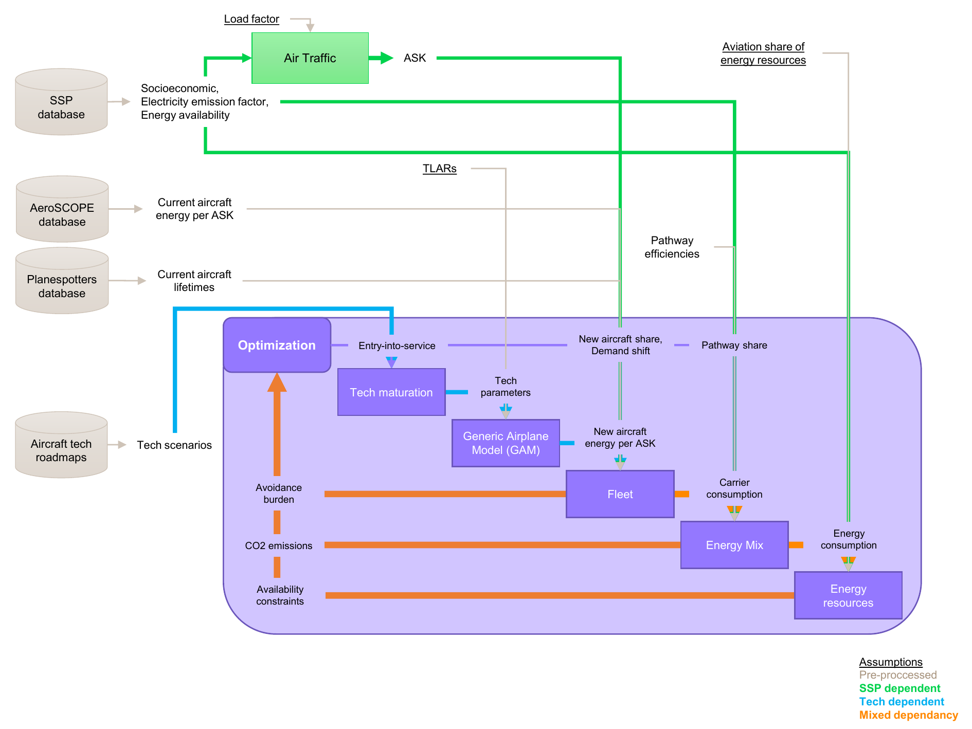
The figure above shows the data-flow between model disciplines and the optimization loop. Before the optimization starts, the chosen global scenario (from the SSP database) determines the evolution of socioeconomic drivers (population and economy) and the energy system (global production of biomass and electricity, and emission factor of grid electricity). Current aircraft data is pre-processed from the AeroSCOPE and Planespotters databases, while technology roadmaps provide component-level performance forecasts.

Then, iteratively, the optimizer chooses a set of policy variables — entry-into- service dates, new aircraft market shares, demand shift, and pathway shares — and the simulation models are evaluated: Air Traffic produces ASK from socioeconomic data, Tech maturation and GAM size new aircraft from technology parameters and TLARs, the Fleet model computes carrier consumption from market shares and aircraft efficiencies, the Energy Mix resolves production pathways into CO₂ emissions, and Energy resources checks availability constraints. The optimizer receives CO₂ emissions, availability constraints, and avoidance burden as feedback to guide the next iteration.

---

1. Models

A Model is the atomic unit: a function that computes outputs from inputs, wrapped as a GEMSEO-JAX discipline.

NOADS provides three base classes:

Class	When to use
AutoModel	Most common. Auto-discovers inputs and outputs from the function signature.
JAXModel	When you need explicit control over input/output names.
Model	Wraps an existing JAXDiscipline directly.

Because every model is a JAX function, gradients are computed automatically via automatic differentiation — no finite differences needed.

A model in practice

from noads.core.model import AutoModel

def my_emission_model(fuel_burn, emission_index):
    co2 = fuel_burn * emission_index
    return co2

model = AutoModel(my_emission_model, name="emissions")

---

2. Scenarios

A TemporalScenario assembles models into a time-dependent optimization problem. It handles:

• Time vectorization: models are evaluated at each time step (2025–2075), but only those with time-dependent inputs are vectorized — constant models are computed once.

• Control interpolation: decision variables are defined at a few time knots and interpolated (linear or cubic spline) to the full time vector.

• ODE integration: first-order delays (technology diffusion, fleet turnover) are solved with diffrax (Dormand–Prince 5).

• Constraint assembly: cumulative carbon budgets, resource limits, and feasibility bounds are collected automatically.

        flowchart TB
    OPT[Optimizer<br/>GEMSEO + SLSQP] -->|control knots +<br/>scalar variables| Interp

    subgraph TS[TemporalScenario]
        direction TB
        Interp[Control interpolation<br/>to yearly time vector]
        ODE[ODE integration<br/>first-order delays]
        Models[Model chain<br/>traffic + fleet + energy]
    end

    Interp --> ODE --> Models
    Models --> Obj[Objectives & constraints<br/>cumulative CO₂, cost,<br/>availability, avoidance]
    Obj -->|objective +<br/>constraints| OPT
    

The optimizer decides the control knots (time-dependent shares, demand shift) and scalar optimization variables (entry-into-service dates) to feed into the TemporalScenario. Inside the scenario, controls are interpolated to the yearly time vector, then first-order delay ODEs are integrated (fleet turnover, technology diffusion), and the resulting delayed controls are passed to the model chain (traffic, fleet, energy). The scenario returns objectives and constraints back to the optimizer for the next iteration.

For robust optimization across multiple climate futures, a MultiScenario vectorizes a TemporalScenario across several SSP pathways and can aggregate outputs (e.g., mean cumulative emissions across scenarios).

---

3. Fleet

The fleet module models aircraft operating in five market segments (general, commuter, regional, short–medium haul, long range):

• AircraftOperation: an existing aircraft type with known energy consumption, propulsion system, and lifetime. The current fleet is initialized from the AeroSCOPE and Planespotters databases.

• AircraftDesign: a new aircraft whose performance is estimated by the Generic Airplane Model (GAM), a physics-based sizing tool. Each design is sized at a given entry-into-service year (EIS, an optimization variable), which determines which technology generation is available. Technology parameters (battery density, motor power, structural efficiency) evolve over time via AircraftTechParameter.

• Fleet: aggregates multiple aircraft competing in the same market. It receives from the optimizer the EIS and maximum market share (\(S^\max\)) of each aircraft type and computes market shares over time via ramped pulse inputs to a first-order delay ODE, accounting for demand avoidance and fleet turnover.

        flowchart TB
    OPT[Optimizer] -->|EIS per aircraft<br/>per market| AD
    Tech[Technology<br/>parameters<br/>2020 → 2040 → 2060] --> AD

    subgraph Designs["Aircraft designs (one per architecture × market)"]
        AD[GAM sizing<br/>at EIS]
        AD --> JetA_GT[JetA-GasTurbine<br/>v1 & v2]
        AD --> lH2_GT[lH2-GasTurbine]
        AD --> lH2_FC[lH2-FuelCell]
        AD --> BatE[Battery-Electric<br/>General + Commuter only]
    end

    JetA_GT & lH2_GT & lH2_FC & BatE -->|energy per ASK| FA
    OPT -->|S_max per aircraft<br/>per market| FA

    AO[Current aircraft<br/>AeroSCOPE] -->|energy per ASK<br/>+ lifetime| FA
    AT[Air Traffic] -->|ASK per market| FA

    subgraph FA[FleetAssembly]
        F0[Fleet — General]
        F1[Fleet — Commuter]
        F2[Fleet — Regional]
        F3[Fleet — Short–medium]
        F4[Fleet — Long range]
    end

    FA --> Cons[Carrier consumption<br/>per energy type]
    

---

4. Energy system

The energy module traces production pathways from primary resources to final energy carriers:

• EnergyCarrier: a fuel or energy medium (kerosene, liquid hydrogen, battery electricity) with physical properties (specific energy, density).

• ProductionPathway: a route to produce energy (e.g., Fischer–Tropsch from biomass, electrolysis from renewable electricity), with associated CO₂, cost, and resource impacts.

• EnergyMix: assembles all pathways and carriers, resolving inter-dependencies (e.g., electricity is both a final carrier and an input to hydrogen production) and computing total system-wide impacts.

        flowchart LR
    Oil[Oil] --> Refinery --> Kerosene
    Bio[Biomass] --> HEFA & FT & ATJ
    HEFA --> Biofuel
    FT --> Biofuel
    ATJ --> Biofuel
    Elec[Electricity] --> Electrolysis --> GH2[Gas H₂]
    GH2 --> PtL[Power-to-Liquid]
    Elec --> PtL
    PtL --> EFuel[E-fuel]

    Kerosene -->|Fossil| JetA[JET-A]
    Biofuel -->|Biofuel| JetA
    EFuel -->|Electrofuel| JetA

    GH2 --> Liq[Liquefaction]
    Elec --> Liq
    Liq --> LH2[Liquid H₂]

    Elec --> Charging --> Bat[Battery]

    subgraph Final[Final energy carriers — embarked in aircraft]
        JetA
        LH2
        Bat
    end
    

---

5. Background scenarios

NOADS does not run in a vacuum — it is driven by exogenous socioeconomic and climate data from the IPCC’s 6th Assessment Report (AR6) [1]:

• SSP pathways (Shared Socioeconomic Pathways): SSP1 through SSP5 provide GDP per capita and population trajectories that drive air traffic demand via a generalized logistic model.

• Carbon budgets: each SSP + temperature target combination (e.g., SSP2-2.6°C) comes with a remaining global CO₂ budget. Aviation’s share is configurable (default ~3%).

• Resource availability: biomass and electricity supply projections bound the feasibility of alternative fuels.

These data are loaded from Excel files in the application/ar6_scenarios_data/ directory and injected into the scenario as exogenous inputs.

---

Putting it all together

A typical NOADS workflow looks like this:

1. Choose a climate scenario (e.g., SSP2-2.6°C, mid-tech).

2. Set up the scenario: single_scenario_setup() builds the fleet, energy system, temporal scenario, design space, and constraints.

3. Run the optimization: GEMSEO drives the SLSQP optimizer with JAX-computed gradients to find the policy trajectory that minimizes cumulative CO₂ (or cost) within the carbon budget.

4. Visualize results: plot emissions, fleet composition, and energy mix over time.

from noads.application.examples import single_policy_scenario_optimization

results = single_policy_scenario_optimization(
    global_scenario_name="SSP2-26",
    technology_index=1,       # mid-tech assumptions
    carbon_budget_percent=3,  # aviation's share of the global CO₂ budget
    plot_optimum=True,
)

For a hands-on walkthrough, continue to the quickstart guide.

---

Software architecture

The diagrams below show the class hierarchy for developers and contributors who want to understand or extend the code.

Core model hierarchy

        classDiagram
    class AutoModel {
      discipline : AutoJAXDiscipline
    }
    class JAXModel {
    }
    class Model {
      discipline : JAXDiscipline
    }
    AutoModel --|> Model
    JAXModel --|> Model
    

Scenario hierarchy

        classDiagram
    class MultiScenario {
      fixed_inputs : list[str]
      mean_outputs : list[str]
      scenario_inputs : list[str]
      scenario_names : list[str]
      temporal_scenario
    }
    class TemporalScenario {
      constant_inputs : list[str]
      constrained_control_groups
      control_delay_times
      cubic_interpolation : bool
      interpolated_inputs : list[str]
      models : list[Model]
      time_integrated_outputs : list[str]
      time_vector
      vectorized_chain : JAXChain
    }
    TemporalScenario --* MultiScenario : temporal_scenario
    

Fleet & energy class diagram

        classDiagram
    class GAM {
    }
    class Fleet {
      consumed_carriers : list[EnergyCarrier]
      models : list[Model]
      operating_aircraft : list[AircraftOperation | AircraftDesign]
    }
    class FleetAssembly {
      fleets : list[Fleet]
    }
    class AircraftDesign {
      mission : Mapping
      power_system : Mapping
      reference_aircraft
      technology_evolution : list[AircraftTechParameter]
    }
    class AircraftOperation {
      energy_per_ask : float
      lifetime : float
      propulsion
    }
    class AircraftTechParameter {
      name : str
      value_2020 : float
      value_2040 : float
      value_2060 : float
    }
    class EnergyMix {
      final_energies : list[ProducedEnergyCarrier]
      impacts : list[Impact]
      input_streams : list[Stream]
      produced_energies : set[ProducedEnergy]
    }
    class ProducedEnergy {
      pathways : list[ProductionPathway]
    }
    class ProductionPathway {
      impacts : list[Impact]
      input_streams : list[Stream]
    }
    class EnergyCarrier {
      specific_energy : float
    }
    class PropulsionSystem {
      energy_carrier_mix : Mapping
    }
    AircraftOperation --* AircraftDesign : reference_aircraft
    PropulsionSystem --* AircraftOperation : propulsion
    PropulsionSystem --o EnergyCarrier : energy_carrier_mix
    ProductionPathway --o Impact : impacts
    ProducedEnergy --o ProductionPathway : pathways
    Fleet --o AircraftOperation : operating_aircraft
    AircraftDesign --o AircraftTechParameter : technology_evolution
    AircraftDesign --o GAM
    EnergyMix --o ProducedEnergy : secondary_energies
    EnergyMix --o Impact : impacts
    AircraftDesign --|> AircraftOperation
    FleetAssembly --|> Fleet