Time-dependent controls#
First-order delays are commonly used to account for simplified inertia regarding: measuring and reporting information, receiving information and decisions being made, and even for decisions to have a visible effect on the state of a system [51, 52]. While the present work automates decision-making based on system outcomes, we still account for delays regarding the time-dependent optimization variables (here called controls). Furthermore, this also allowed for numerical benefits, such as reduced dimensionality and improved the optimization stability.
Each output variable \(o(t)\) is modeled as an Ordinary Differential Equation (Eq. 1), which is dependent on a given input variable \(i(t)\) and a delay-time \(\tau\). Fig. 4 shows the output response of the first-order delay system for a set of inputs. For ramped step input (with ramp duration of \(2\tau\)) it takes \(4\tau\) for the output to reach 95 % of the step value, considered as one replacement lifetime.
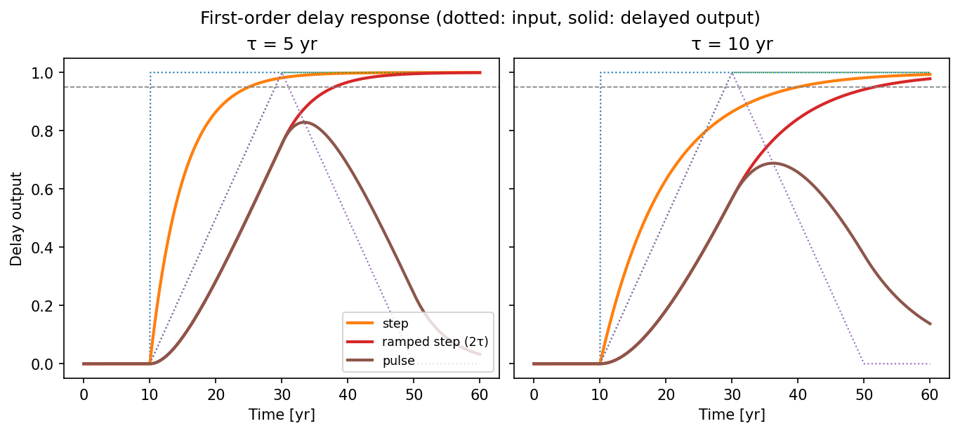
Fig. 4 Response of the first order delay to a set of input paths (step, ramped step, and pulse), for two time constants, subject to initial value of 0.#
The supply shift ratio (Eq. 7) and the shares of pathway production (Eq. 14 and Eq. 16) are modeled with inputs that are coarsely discretized in time (2.5 years, while the simulation step is 1 year), here the input values at each time are optimization variables. The shares of aircraft market penetration are modeled with a ramped pulse, parameterized from 4 optimization variables (ramp start year, max value, lifetime, and ramp-down duration).
Three families of controls are used, each subject to its own feasibility constraint. Fig. 5 to Fig. 7 show, for each, a valid set of optimization variables (one that respects the constraint), as both the control-point inputs (the optimization variables) and the delayed outputs that actually drive the simulation.
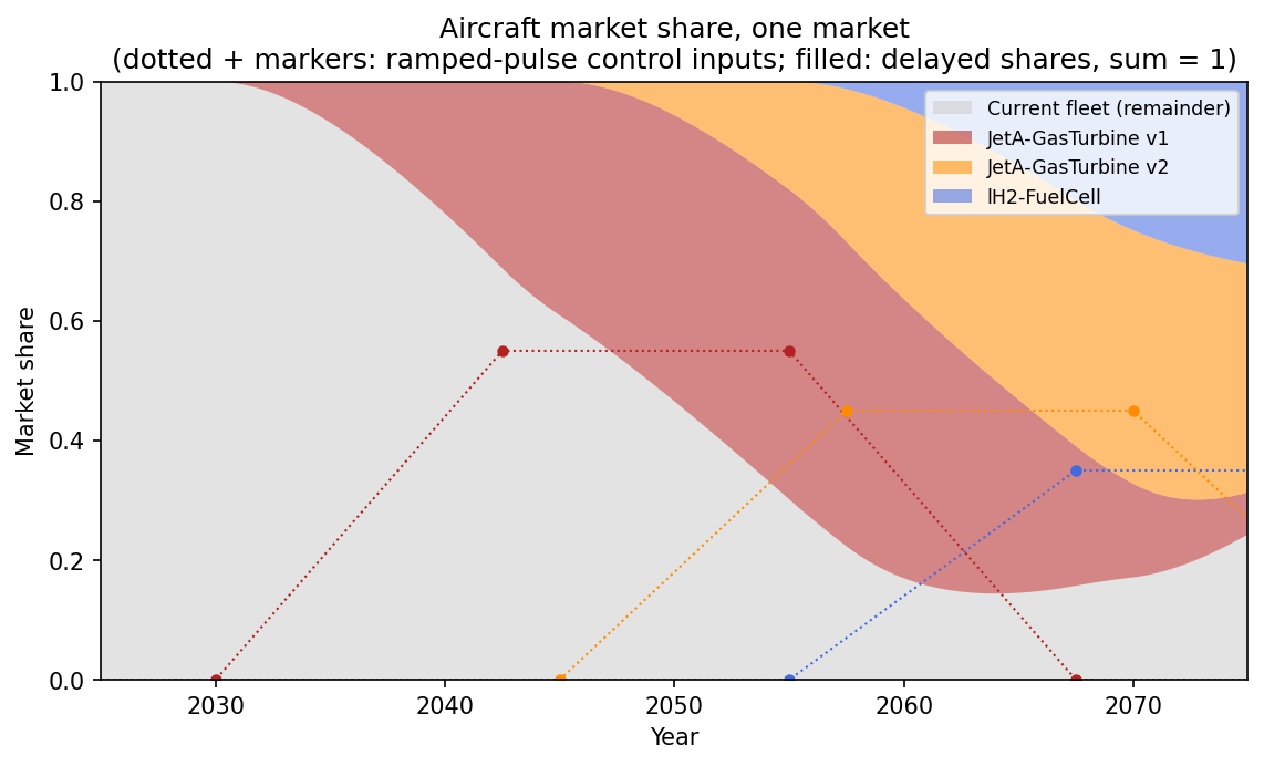
Fig. 5 Aircraft market shares within one market. Each new aircraft is a ramped pulse (entry-into-service, maximum share, lifetime, ramp-down) delayed with \(\tau = \text{lifetime}/4\); the new-aircraft shares sum to at most one at every time, the current fleet taking the remainder (\(1 - \sum\)). Dotted lines with markers are the control inputs; the filled areas are the delayed shares, which fill up to one.#
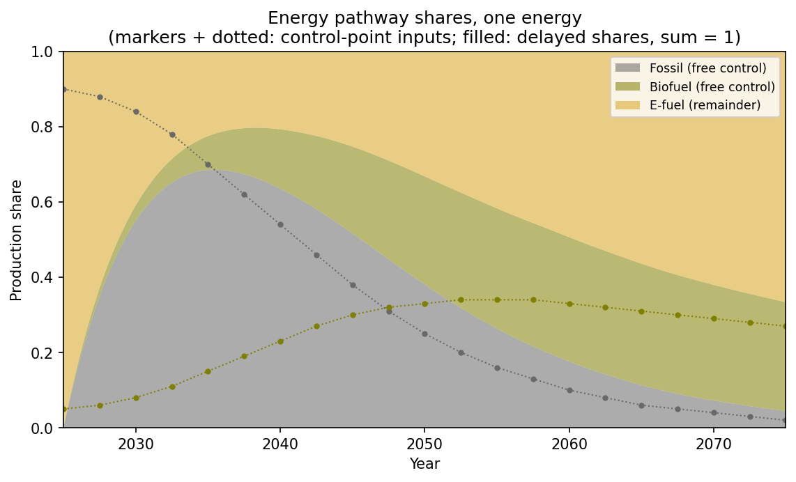
Fig. 6 Production shares of the pathways of one energy. Each non-last pathway is a knot control in \([0, 1]\) (delayed with \(\tau = 5\) yr); the shares sum to one, so the last pathway takes the remainder. Markers and dotted lines are the control-point inputs; the filled areas are the delayed shares.#
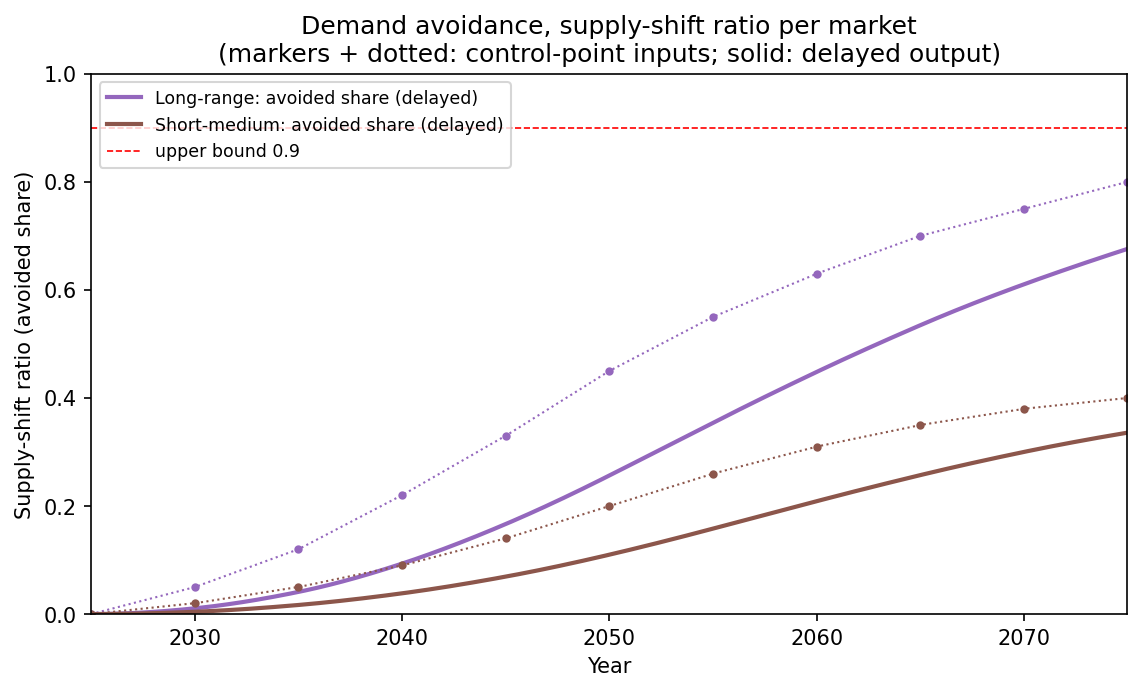
Fig. 7 Supply-shift ratio (avoided fraction of trend supply) for two markets, a per-market control bounded to \([0, 0.9]\) and delayed with \(\tau = 10\) yr. Markers and dotted lines are the control-point inputs; solid lines are the delayed outputs.#
Reproduce these figures#
The delay response and how each kind of control (aircraft market share, energy pathway shares, and demand avoidance) maps the optimization variables to smooth simulation inputs are produced by the following example: