Energy-Mix

This work considers different energy carriers, and for some of them several production pathways are available, such as synthetic fuels. Moreover, some energy carriers can be consumed in the production of other carriers and some of them can compete for the same primary energy sources or materials. In that regards, it is necessary to consider a modular implementation to the energy production model.

Each energy conversion process is modeled in a modular manner as a production pathway. Pathways have a specific consumption of input flows per unitary production of output flows. The energy mix assembles all the production processes and the links them to calculate both intensive and extensive properties of the energy production system.

The computation of the impact generated (only CO2 emissions in this work, but any cumulative impact could be extended, such as land required, water consumption, …) per unitary production, an intensive quantity, is made from primary-to-final. This is mainly due to the fact that the impacts made in the production of inputs must be known beforehand in order to be accounted for in the indirect impacts of outputs. On the other hand, the aggregated consumption and production of energies, an extensive quantity, is made from final-to-primary, because total consumption of final energies determine the required consumption of inputs, which determines how much production of each energy-input is required.

In some implementations of modular energy system models, the estimation of properties is made altogether (intensive and extensive) per energy type and pathway [30]. This creates a coupled model: intensive quantities depend on the mix of the upstream system and extensive quantities depend on the aggregated consumption of the downstream system. This yields that an initial guess must be made up- and downstream, which is then iteratively solved until convergence. By separating modules responsible for estimating intensive and extensive quantities, if the system has no retroaction, the coupling disappears and direct computation can be achieved.

Intensive impacts

Table 5 Energy consumption and direct emissions for each of the production pathways considered. For pathways under technology maturing, the two values represent the 2025 and 2050 values.

Energy Carrier	Production Pathway	Oil (MJ/MJ)	Biomass (MJ/MJ)	Electricity (MJ/MJ)	Gas H2 (MJ/MJ)	Direct emissions (g CO2 / MJ)	Source
Fossil Jet-A	Refinery	1.16				88.7	[39]
Biofuel	HEFA		1.95			62.73	[40]
Biofuel	ATJ		3.33			51.55	[40]
Biofuel	FT		5.0			35.3	[40]
Gas H2	Gas reforming					101.5	[80]
Gas H2	Electrolysis			1.41-1.33		0	[41]
Electrofuel	Power-to-liquid			0.65-0.56	1.89-1.68	0	[41]
Liquid H2	Liquefaction			0.22-0.16	1.0	0	[41]

Impacts generated in the production of energy carriers are heavily dependent on the efficiency of processes and the impacts of consumed inputs, and these are mainly determined by the background energy system [81]. Recent works have highligthed the importance of linking global scenarios to perform prospective life-cycle assessment of energy [82], and have also been applied for the prospective assessment of climate neutral aviation [83], showing a great increase in emissions associated with the production of synthetic jet fuel when a 3.5°C temperature increase scenario is chosen instead of a 2°C one.

The impact factor \(IF_{\text{pathway}}\) (Eq. 13), impact per unitary production, of each output flow associated to production pathways is modeled as the sum of direct impact generated at production plus the impacts associated to the input flows consumed in the process. \(CF_{p, i}\) is the consumption of input \(i\) per unitary production of pathway \(p\). This is made because the inputs consumed in the process have impacts themselves, and by consuming them these indirect impacts must be accounted in the impacts of the output flow.

Table 5 summarizes the production pathways for each of the accounted energy carriers, their energy consumption and direct emissions per produced output. Technology maturing was accounted for some production pathways with an inverse consumption (analogous to process efficiency) that decreases linearly until stagnation in 2050.

(13)\[\begin{split}\begin{aligned} IF_{\text{pathway}}= & IF\text{direct}_{\text{pathway}}\\ &+\sum_{i\ in\ \text{pathway inputs}}CF_{\text{pathway}, i}\ IF_i \end{aligned}\end{split}\]

(14)\[IF_{\text{energy}}=\sum_{p\ in\ \text{energy pathways}}S_p\ IF_p\]

Because each energy type can be produced by several pathways, a mixing process is applied where the energy mean impacts \(IF_{\text{energy}}\) (Eq. 14) is weighted by the share of pathway production, which are treated as a time-dependent control, used as optimization variables.

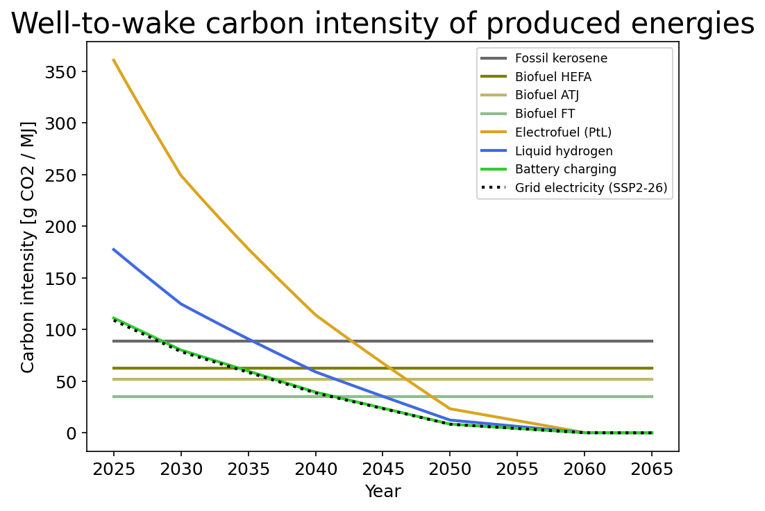
Fig. 15 Well-to-wake carbon intensity of the produced energies under the SSP2-2.6 background scenario. Fossil kerosene and biofuels have carbon intensities that are constant in time, whereas the electricity-based carriers (electrofuel, liquid hydrogen, battery charging) decarbonize together with the background grid and with maturing process efficiencies.

Fig. 15 shows how the resulting carbon intensity of each produced energy evolves over time: fossil kerosene and biofuels stay constant, while the products derived from grid electricity follow the decarbonization of the background scenario down towards near-zero carbon intensity.

Extensive production and consumption

The production of each energy type (Eq. 15) is the direct energy consumption (directly embarked in aircraft) plus what was consumed to make other energy types. If \(e_0\) is an energy input to \(e_1\), \(e_1\) is an energy output to \(e_0\). The computation is initialized with final energies because the term \(\sum_{o}(CF_{o, e}\ P_o)\) is zero, as no intermediate processes consume them.

(15)\[P_{\text{energy}}=C\text{direct}_{\text{energy}} + \sum_{o\ in\ \text{energy outputs}}CF_{o, \text{energy}}\ P_o\]

(16)\[P_{\text{pathway}}=S_{\text{pathway}}\ P_{\text{energy}}\]

The production of each pathway (Eq. 16) is then estimated from pathway share. Input consumption of pathways are estimated (Eq. 17) and then are aggregated by energy type (Eq. 18). The process is then repeated for each energy type until primary energies.

(17)\[C_{\text{pathway}, \text{input}}=CF_{\text{pathway}, \text{input}}\ P_{\text{pathway}}\]

(18)\[C_{\text{energy}, \text{input}}=\sum_{p\ in\ \text{pathways}} C_{p, \text{input}}\]

Consumption and impacts constraints

For biomass and electricity, the total consumption is constrained applying the concept of an allocation principle, initially developed for Absolute Environmental Sustainability Assessments [84, 85], but applied for energy production (Equation Eq. 19). Because there is little consensus on how to find such fair shares [86], two different values were explored: one reflecting a conservative energy availability (5.0 %), and another reflecting a preferential availability to the aviation sector (8.6 %). Both values use some sort of grandfathering, which tend to lock the economic system into its present state. Yet, values are still conservative when compared to other institutional roadmaps [2].

(19)\[C_{\text{resource}} \le s_{\text{resource}} P_{\text{resource}}\]

The conservative value was obtained based on a reference mitigation scenario, the IMP-REN-2.0, in which 38.6 % of the biomass production is allocated to the transport sector [87], the fair share allocated to aviation is considered to be 13 % of that, which is the 2019 sector’s share of oil consumption relative to the entire transportation consumption [88]. The preferential access value was obtained based on the sector’s 2019 share of global oil consumption [88].

(20)\[\int_{t_0}^{t_1} CO_2(t) dt \le s_{CO_2} B_{CO_2}\]

In the low demand formulation, the cumulative emissions of the sector is a constraint rather than the objective to minimize (Eq. 20). In these cases, we assumed the target carbon budget \(B_{CO_2}\) to be the remaining 2°C carbon budget with 66 % confidence [89], and the fair share to be 3.0 %, which is the sector’s share of direct, indirect and induced GDP [90].

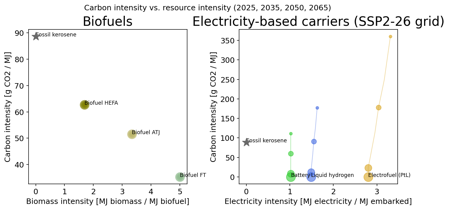
Fig. 16 Trade-off between carbon intensity and resource intensity for the produced energy carriers, evaluated at 2025, 2035, 2050, and 2065 (marker size grows with the year), with fossil kerosene shown as the reference (star). For biofuels the trade-off is static: lower-emitting pathways (FT) consume more biomass than higher-emitting ones (HEFA). For the electricity-based carriers the operating point moves down and to the left over time as the background grid decarbonizes and the conversion processes mature.

Fig. 16 makes the two resource trade-offs explicit. Relative to fossil kerosene, biofuels reduce carbon intensity only by consuming biomass, and the pathways that emit least (Fischer-Tropsch) are the most biomass-intensive. The electricity-based carriers instead trade grid electricity for carbon intensity, and both their electricity intensity and their carbon intensity fall over time; electrofuel remains the most electricity-intensive route because it chains electrolysis, power-to-liquid, and the upstream grid.

Reproduce these figures

The energy production system and the aircraft energy efficiency figures are produced by the following script:

Energy production system

Energy production system