Models

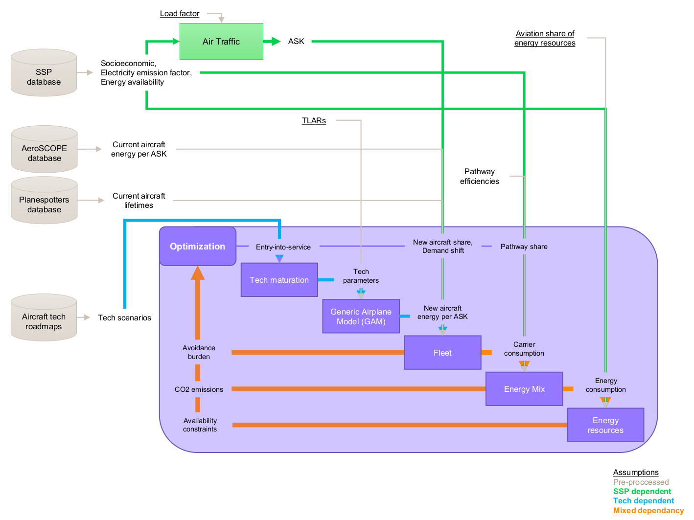
Fig. 2 Conceptual view of the optimization process and data-flow between modeled disciplines.

An overview of the data-flow between the model disciplines is presented in Fig. 2. Before the optimization loop starts, the chosen global scenario determines the evolution of socioeconomic drivers (population and economy) and energy system (global production of biomass and electricity, and emission factor of grid electricity). Then, iteratively a set of policy variables is chosen (when and how much to deploy new aircraft, how much to produce of energy pathways, how much of trend traffic to avoid) and the simulation models are evaluated for estimating objective, and constraints for a given optimization formulation.

The numerical methods employed to accelerate optimization for nonlinear and time-dependent policy analysis were crucial to enable fast multi-scenario analysis. These include: automatic model coupling, constrained gradient-based optimization algorithms, automatic differentiation, vectorization, and compilation (see Numerical methods).

An overview of the models and assumptions behind scenario generation is provided in Table 1, the following pages provide the detailed explanation on assumptions, model equations, comparison with related works, and calibration methodology (supplementary information of the published article).

Table 1 Main assumptions for of the model disciplines.

Model discipline	Assumptions	Limitations
Policy controls	Policy variables act on fleet replacement (per aircraft per market) and energy production shares (per pathway), the low-demand formulation also includes a cap in supply (per market). Controls evolve gradually in time subject to a linear delay.	Time-delayed share-based control creates instability under rapid production volume changes.
Air traffic demand	Future trend Revenue Passenger Kilometers (RPK) demand estimated based on scenario-dependent population and income per capita [1]. Demand grows with income, but is assumed to saturate at around 2700-4300 pax-km/capita (scenario-dependent) and represented via sigmoidal (logistic-type) functions calibrated on historical data. The supply, in terms of Available Seat Kilometers (ASK), is then estimated using a quadratic load factor [20, 33] that grows from 84.4 % (2019) to 92 % (2075).	Prospective analysis uses logistic functions outside range of calibrated data, problematic for estimating saturation levels of developing countries. Global aggregation ignores regional disparities. Price elasticity not coupled with energy costs.
Current aircraft	The initial fleet composition and performance are fixed and calibrated to historical data [34, 35]. Fleet parameters (efficiency, lifetime) are exogenous and differentiated by market segments, but may vary due to technology assumptions.	Potential mismatch between current efficiency (aggregated by flight distance) and aircraft lifetimes (aggregated by number of seats).
New aircraft	Generic Airplane Model (GAM) [36] for conceptual design of future aircraft with conventional and alternative propulsion architectures, such as: (i) conventional kerosene turbofan, (ii) liquid-hydrogen turbofan, (iii) liquid-hydrogen fuel-cell and electric motors, and (iv) battery-electric aircraft. Aircraft are designed for market-specific missions, and deployed by Entry-Into-Service (EIS) year, which are also optimization variables (per market per aircraft). Technology maturing is incorporated with assumptions component-level performances (structures, batteries, cryogenic tanks, fuel cell, …) that varies in time and according to technology assumptions, reducing energy consumption at later EIS.	TLAR fixed within markets (size, speed, altitude not optimized). Cryogenic tank efficiency fixed across markets, ignoring size dependency [12, 37]. Gas turbine weight and consumption assumed identical for kerosene and hydrogen [38].
Fleet replacement	Current aircraft is replaced by new aircraft types, designed specifically for market range. Replacement is gradual with market-specific lifetimes of 15.3-33.8 years (variable with technology assumptions).	Airlines may operate aircraft at shorter distances than designed mission, increasing fuel consumption beyond modeled values.
Energy mix	Aviation energy demand may be supplied by a mix of different energy carriers (Jet-A fuel, Batteries, Liquid-hydrogen), each of them being produced by different production pathways (fossil kerosene, biofuels, e-fuels, electrolysis, …). Well-to-wake (WTW) lifecycle emissions are considered for all carriers, with constant in time carbon intensities for kerosene and biofuels [39, 40], while electricity-based pathways have emission intensities calculated based on process efficiencies [41] and scenario-dependent grid emission intensity.	No differentiation between biomass types (all pathways compete for same resource). PtL consumption assumes only Direct Air Capture as source for carbon, concentrated CO2 sources are not considered [42].
Constraints	Feasibility is evaluated with: initialization constraints (each aircraft must be feasible by EIS), and path-wise constraints (current fleet retirement per market, pathway-mix per carrier, fair share of biomass and electricity consumption), the low-demand formulation also includes an end-time constraint (cumulative emissions).	Fair shares of global production allocated to aviation estimated with grandfathering approaches based on energy consumption.
Objectives	Minimize cumulative emissions (trend formulation), or minimize discounted relative price increase due to supply-cap (low demand formulation).	Simplified modeling of relative price increase with constant price elasticities among markets.

Model preamble

In earlier studies [24], models primarily aimed to link SSP scenario data and aircraft design routines within an aviation system model, through a direct re-implementation of AeroMAPS equations [20]. The new models and numerical methods developed in this work will subsequently be re-incorporated into AeroMAPS.

The energy inputs consumed to meet the necessary final energy carrier production and the emissions generated are estimated from process efficiencies, direct emissions from pathway production and grid electricity emission factor linked to a global scenario. In the present model, each biofuel pathway competes for the same biomass feedstock, considering direct emissions and process efficiencies as an average of the different feedstock-specific processes [40]. However, this approach represents a simplified view, since each biofuel pathway can actually consume specific feedstocks, such as energy crops (competing with food production), oil-based feedstocks and wastes. For example, HEFA biofuels can be obtained from oil-based feedstocks (such as jatropha and camelina), but also from used cooking oil. The final climatic impact of biofuels also depends on potential land use change, especially in the case of competition with food production [43].

The modeling of costs (energy, aircraft, operations) is outside the scope of this paper. Under the current production system, the price of alternative energy carriers is higher than that of fossil kerosene [44, 45], but this gap is expected to decrease in the near future due to scaling of production and due to carbon pricing [46], especially in scenarios with ambitious climate targets.