Air traffic demand#
In order to account for the phases of growth, maturation and saturation observed in aviation demand [53], a generalized logistic function is used to estimate trend per-capita demand from per-capita income. This model explicitly accounts for saturation of per-capita transport demand as per-capita incomes grow, differently to the approach in most IAMs, which rely on extrapolations [54] or assumptions of constant income elasticity [29, 55].
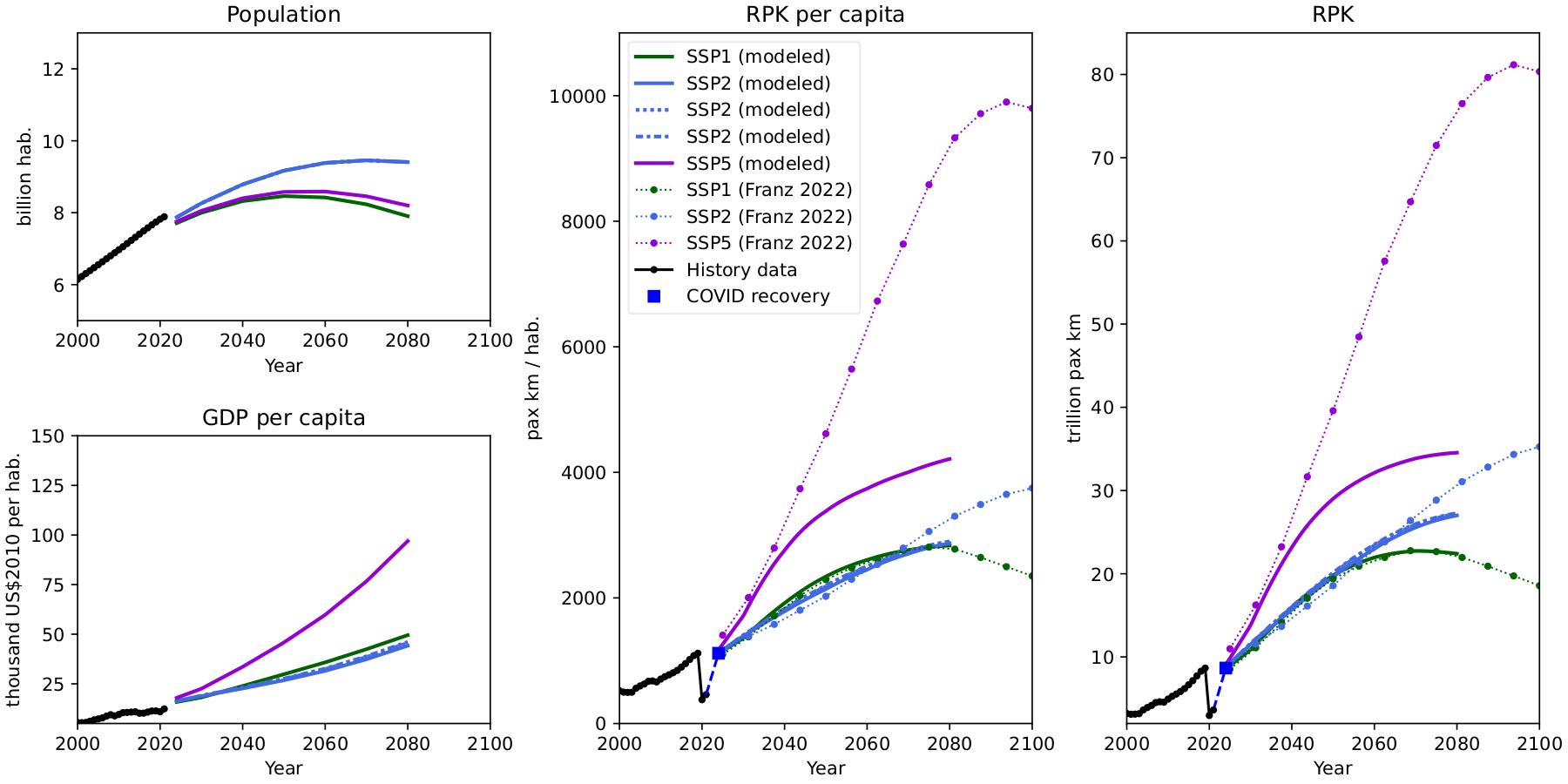
Fig. 8 Historical evolution and modeled future global RPK demand from socioeconomic drivers linked to SSP scenarios. Results are compared with [54]. Explicitly incorporating per-capita demand saturation (current model) yields much lower traffic levels in the long term, when compared with models based on the extrapolation of short term income elasticities.#
Fig. 8 shows the recent history and SSP scenario future evolution of Population and GDP per capita, and also the recent history and modeled future global RPK demand. SSP2 follows the historically calibrated logistic function, demand grows with varying pace due to income growth, but stabilizing at around 3000 passenger-kilometers per capita. SSP1 displays high initial growth due to income, but stabilizes demand sooner and 90 % lower than trend; while for SSP5 growth is sustained at even higher pace, and stabilize at much higher levels of around 4300 passenger-kilometers per capita, 50 % higher than trend. For comparison, crossing AeroSCOPE [34] and World Bank [56] averaged 2019 traffic per capita for multiple countries: India is 198, China 902, Brazil 959, World 1377, Japan 2669, France 3561, Germany 3718, and USA 6974.
As highlighted in the assessment by Frank et al. [54] when estimating demand there is also the need of endogenizing SSP narratives beyond accounting for scenario-specific GDP and population growth, a proposition is also made for incorporating voluntary demand restraint (for SSP1 scenarios) or incentives (in SSP5 scenarios) as well as an extra policy measure of market-specific demand caps for dealing with strict carbon budget constraints. Comparing these results with the ones generated by the present work, SSP1 shows a very close agreement both in terms of per-capita traffic as for total demand, SSP2 shows close agreement up until 2070, after that the logistic model employed yields lower per-capita traffic than Franz’s model, with declining income elasticities. This disagreement is further intensified in SSP5, even with the higher stabilization traffic levels.
Detailed formulation#
Many drivers can be linked to the growth in air traffic demand: population, disposable income, trade volumes, fuel prices, urbanization [57].
Equation Eq. 2 presents the model used in the Global Change Analysis Model (GCAM) [29, 55], where \(Pop\) is population, \(I\) is per-capita income, \(p\) is ticket price, \(\epsilon_{\upsilon}\) is the elasticity of demand to variable \(\upsilon\), and \(\sigma\) is a calibration constant. Yet, there are several issues with using constant elasticities for forecasting aviation demand over long time-horizons. Meta-analyses categorize it as a luxury good and immature market [58], and post-COVID studies demonstrate how income elasticities may change rapidly depending on the state of the business cycle (normal, downturn, recovery) [59].
In the context of general transportation, these models are also limited to account for demand saturation as personal incomes rise, resulting in ever-growing demand volumes as the Gross Domestic Product (GDP) grows, and that by using S curves (Logistic, Gompertz, or Richards sigmoid functions), to account for the income effect, can produce better estimates for both developed and developing countries [60]. This method was first applied for estimating personal vehicle stocks from personal income [61]. Results show that income elasticities can vary significantly as countries develop, but one shortcoming of the model is ignoring the effect of prices in modifying the demand.
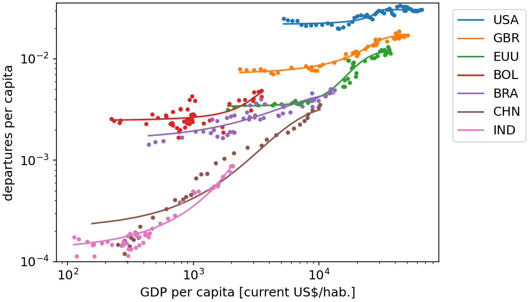
Fig. 9 Regional calibration of registered carrier departures per capita as a generalized logistic function of income per capita. Region code: GBR - United Kingdom, USA - United States of America, EUU - European Union, BOL - Bolivia, BRA - Brazil, CHN - China, IND - India. Data from [56].#
In order to account for the phases of growth, maturation and saturation observed in aviation demand [53], a generalized logistic function is used to estimate trend per-capita demand from per-capita income. In Equation Eq. 3, \(L\) and \(R\) are the left and right asymptotes (personal propensity to travel at \(0\) and \(\infty\) personal income), \(\iota\) is the income per capita at the inflection point, \(B\) is the logistic growth rate, \(C\) controls the duration of the transition from \(L\) to \(R\), and \(\nu\) controls near which asymptote maximum growth occurs (\(\nu=1\) would yield an logistic equation and \(\nu\to0^+\) would tend to a Gompertz function).
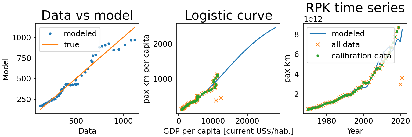
Fig. 10 Calibration of global per capita RPK demand as a generalized logistic function of per capita GDP. Data from [56, 62].#
The parameter set \(\theta=(L, R, \iota, B, C, \nu)\) must be calibrated with historical data. In the regional calibration, World Bank data [56] provided for the demand (carrier departures), population, and income proxies on a regionalized level. But as the traveled distance is highly important in determining total emissions, in the present work, mitigation scenarios are driven by RPK demand, therefore ICAO data was used and calibrated on a global level over the 1980-2019 period. COVID years were excluded from the calibration data, and its after-effects were considered by assuming that by 2024 per capita traffic will reach 2019 levels, this is achieved shifting the parameter \(\iota\) by the gap in income per capita between 2024 and 2019.
The coefficients were calibrated to minimize the 2-norm of the error, resulting in error to data ratio[1] of 10.6 %. This yields an R2 of 0.954 over the per capita data, and 0.967 over the globally aggregated data, which was considered sufficient for the global prospective analysis carried. Fig. 10 shows how the calibrated model compares to historical data, the error distribution, the resulting logistic function, and the global RPK time-series.
Besides the logistic trend calibrated based on historical relationships, scenario narratives are further endogeneized by accounting a storyline multiplier factor to trend demand (Eq. 4), which is essentially another S-curve that goes from 1 to \(F_{SSP}\) with inflection at around 1.5 times 2024 income per capita. For SSP scenarios 2, 3, and 4 \(F_{SSP}=1\), meaning they will follow the historically calibrated logistic function. For scenario 1, \(F_{SSP}=0.9\) stabilizing demand 90 % lower than trend; while for scenario 5 \(F_{SSP}=1.5\).
The supply, in terms of ASK, is then estimated using Load Factor (Eq. 6) that grows following a quadratic curve in time [33] from 82.4 % in 2019 to 92 % in 2075.
Reproduce these figures#
The demand calibration and the SSP scenario projections are produced by the following scripts:
Calibration of air traffic demand models: global and regionalized