Aircraft and fleet

Aircraft and fleet#

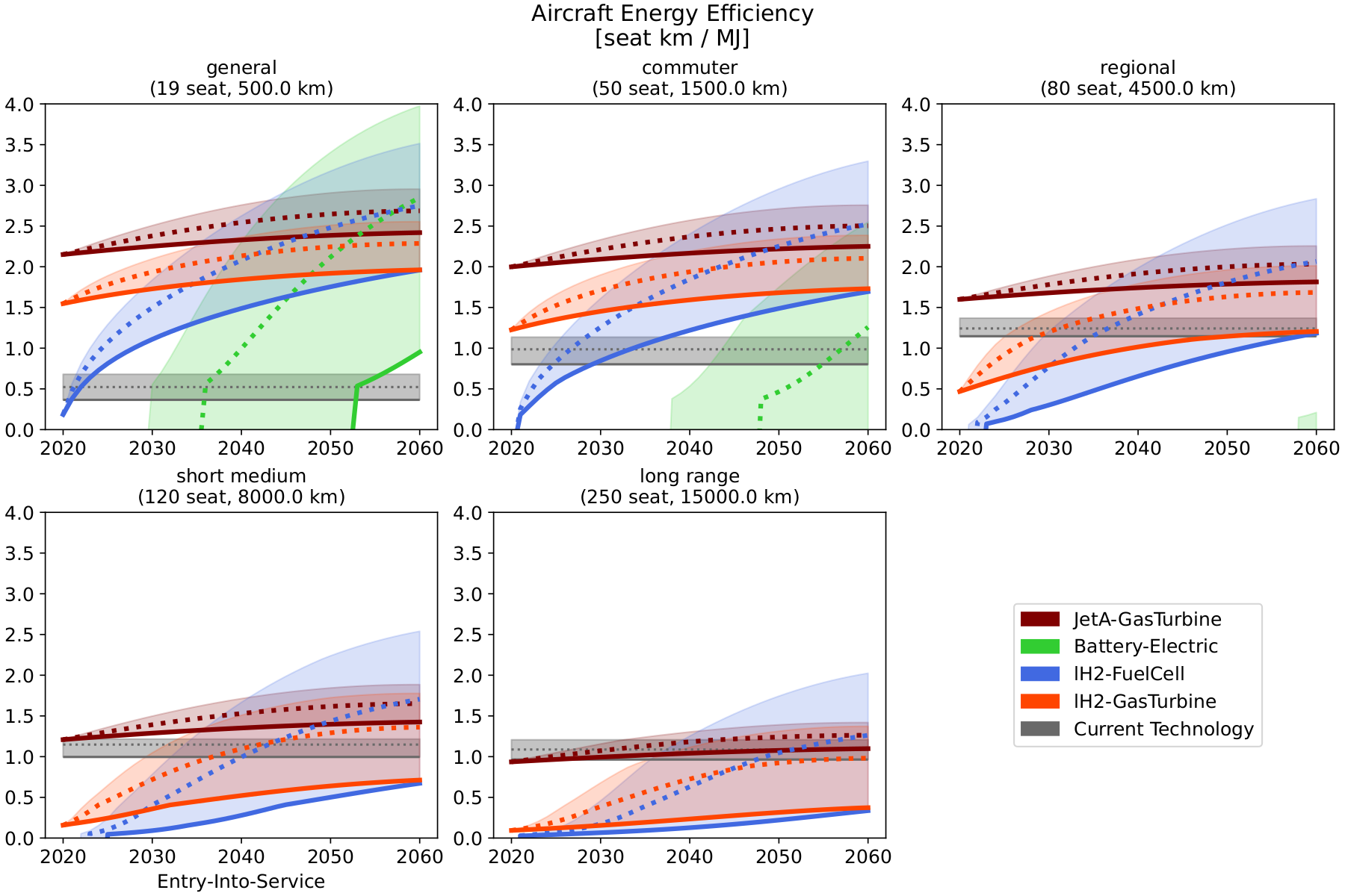
../../_images/aircraft_prospective_energy.png — Fig. 11 Expected passenger efficiency (inverse energy consumption) of prospective aircraft with technology available by Entry-Into-Service. Color-code is used to differentiate among aircraft architectures, filled between the upper and lower limit for the technology scenarios, solid line shows Lower technology scenario, dotted line shows Mid technology scenario. The grey horizontal lines shows the values initialized for the current technology, estimated based on the 3 quartiles (Lower: 1st quartile, Mid: median, Upper: 3rd quartile) of 2019 flights within market distance-bands [34].#

Aircraft design#

Fig. 11 shows the expected design performance of aircraft design architectures depending on prospective technology scenario. Energy consumption of new designs are compared with the 3 quartiles of 2019 commercial flights operated within the category distance bands, obtained from the AeroSCOPE dataset [34].

Conventional aircraft

In general, new conventional gas turbine designs, powered by Jet-A perform better than the mean 2019 fleet, and this gap is wider over smaller distances. The diverging expectations in weight reduction expectations, yield a variation in the energy consumption of these designs depending on the chosen technology scenario, but this variation is relatively small compared to that of alternative designs.

Electric aircraft

Due to the low specific energy of batteries compared to other energy carriers, electric aircraft are still limited in range. Performance varies greatly with technology scenario, due to variation of batteries, electric motors, and power electronics.

Low technology yields that feasible designs in the general market are only possible around 2050. With Mid and Upper technology, respectively, feasibility can be achieved by 2037 and 2032 in the general market, and by 2046 and 2038 in the commuter. By 2060, with Upper technology, electric aircraft is the most efficient for the general market.

Hydrogen aircraft

Hydrogen aircraft are feasible across all markets regardless of EIS, both for architectures that burn hydrogen in gas turbines as for using them with fuel-cells and electric motors. Technology scenario affects them more than conventional aircraft, but less than electric. The sensibility regarding technology scenario is due to the gravimetric efficiency of liquid fuel tanks, but the fuel cell architecture displays higher sensitivity, also due to electric motors and fuel cells (both in terms of efficiency and specific power).

With Lower technology, burning hydrogen in gas turbines is more efficient than using fuel cell for all markets, regardless of EIS. In the general and commuter market, as early as 2030 both are already more efficient than the reference 2019 aircraft. In the regional market, this shift happens by early 2034 and 2042, respectively. In the short-medium, by 2044 and 2050. But neither of them are able to reach 2019 efficiencies in the long-range even by 2050.

With Mid technology, fuel cells surpass combustion around 2040, a bit earlier for shorter distances and a bit later for longer distances. Within the time-frame, both are able to surpass 2019 efficiencies, but neither are able to surpass the efficiency of turbofan architectures.

Finally, with Upper technology hydrogen combustion is able to reach the Lower efficiency of conventional designs. Also with Upper technology scenario, fuel cells are the most efficient option among architectures, except for the general market, but this supposes switching membranes with low temperature operation to high temperature [63].

Current aircraft fleet#

Figures: 2019 flight histograms

(To be added: figures/figs_models/histogram_ask.png and figures/figs_models/histogram_co2.png — histograms of ASK and CO2 emissions for 2019 flights according to flight distance; the black vertical lines show how the market segments are separated. Data from [34]; requires the AeroSCOPE per-route dataset, which is not distributed with the repository.)

The main properties of the current aircraft fleet are initialized based on data from the AeroSCOPE database [34]. The database contains information (passengers flown, seating capacity, fuel burn, emissions) for each origin-destination route for the year 2019 (flight histograms). This is then used in order to estimate the share of global traffic per market segment (supposed to stay constant in time), and also the energy consumption of a typical aircraft within a market.

It is further assumed that, within a given market segment, aircraft can only be replaced by a new aircraft architecture tailored for this market. As shown in Fig. 12, there are significant discrepancies in the aircraft passenger efficiency (the inverse of the energy consumption per seat-km) for flights within the same market segment, and which are higher over short distance flights, meaning that aircraft used for these are not optimized for these distances.

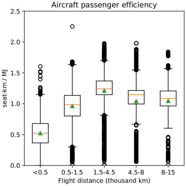
../../_images/current_aircraft_energy.png — Fig. 12 Distribution of current passenger efficiency according to flight distance. Data from [34].#

To account for this, the energy consumption initialized for the current fleet is dependent on the technology scenario: the Lower technology considers the lower quartile in terms of passenger efficiency, the Mid technology considers the median, and the Upper technology considers the upper quartile.

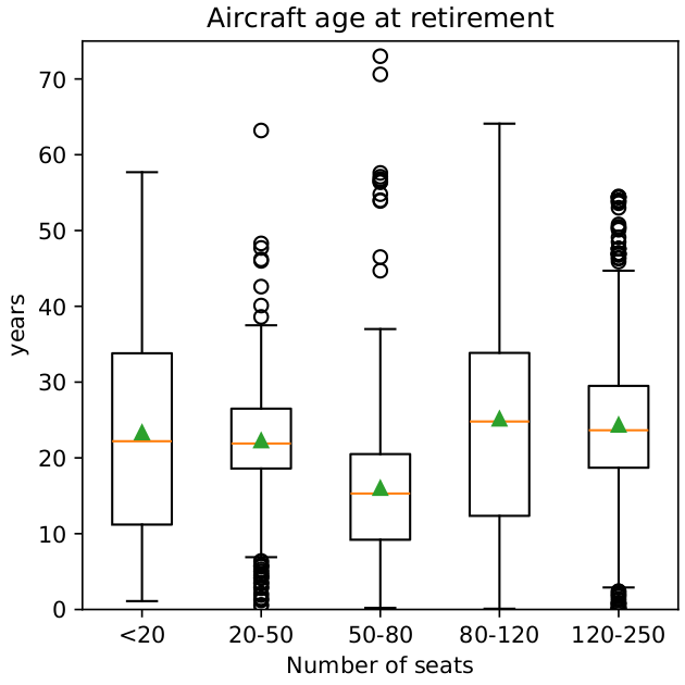
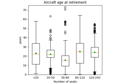
../../_images/current_aircraft_lifetime.png — Fig. 13 Distribution of aircraft age at retirement according to number of seats. Data from [35].#

At last, the lifetime of the current aircraft fleet are initialized based on data from the planespotters database [35]. Instead of aggregating market segments based on distances, aircraft are aggregated by number of seats for closer alignment with aircraft design classes, and it is assumed that, within a market aircraft are subject to the same fleet replacement dynamics. Fig. 13 shows how the age of retired aircraft is distributed, within each segment the distribution is positively skewed (median is lower than mean), but there are significant discrepancies within and across markets. The fleet lifetimes are also dependent on technology scenario: the Lower technology considers the upper quartile in terms of lifetime, the Mid technology considers an intermediate value, and the Upper technology considers the median value. The lower quartile is not used, as the median value is already below the mean, and therefore already a more optimistic value than currently. For comparison, values used for fleet replacement lifetimes in analogous studies [16, 64, 65] are, respectively, 15, 20, and 25 years.

Table 2 TLAR determined by market segment.#
Market	Range (km)	Seats	Consumption (MJ/seat-km)	Lifetime (years)
General	500	19	2.74-1.47	33.8-22.2
Commuter	1500	50	1.25-0.88	26.5-21.9
Regional	4500	80	0.87-0.73	20.5-15.3
Short-medium	8000	120	1.00-0.82	33.8-24.8
Long range	15000	250	1.03-0.83	29.5-23.6

Table 2 summarizes how market segments are split into aircraft range and number of seats, as well as the assumptions on vehicle consumption and lifetime initialized for the market (the last two being dependent on the technology scenario chosen).

Prospective aircraft design#

Modifying the energy carrier changes and the propulsion system architecture requires specific technology, e.g., cryogenic fuel tank, fuel cells, electric motors, all of which are expected to mature at different rates.

To demonstrate this, several sources are used to provide technology parameters and expected year of entry-into-service, which include research papers on green transportation technologies [23, 41] technology roadmaps from IATA [66] and ATI [37, 63, 67, 68], ICCT aircraft design studies [13, 14, 15] NASA electric propulsion studies and technology aspiration [69, 70, 71, 72] and EASA type certificate data [73].

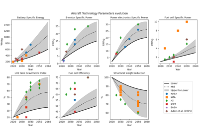
Table 3 presents the lower and upper values used for the technology parameters, according to entry-into-service (EIS) and Fig. 14 displays how some key parameters are interpolated in time and how they compare with the sources used. The main goal of this is to be able to account for the trade-off regarding the timing of deployment of aircraft architectures: early deployment of maturing technology and lock-in with mediocre performance, or late deployment with mature and better performances. Fig. 14 compares the values used in the present work with the literature depending on expected year of Entry-Into-Service.

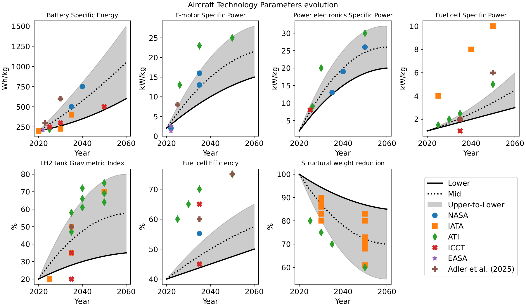
../../_images/aircraft_technology.png — Fig. 14 Improvement in selected aircraft parameters as a function of expected Entry-Into-Service. Filled between the upper and lower limit for the technology scenarios, solid line shows lower technology scenario, and dotted line shows mid technology scenario.#

In order to avoid over-reliance on optimist technology, especially in a sector that has missed many of its recent environmental targets [74], some sources that are purposefully left out of the technology scenario range. This is of particular importance for fuel-cell systems because:

Fuel-cells have limited power output, so several cells have to be stacked to compose total power, decreasing power-to-weight ratio of the system;
Narrow ranges of operating temperature plus high thermal losses, means these systems require thermal management for high-power applications, adding further weight (which is included in the fuel-cell specific power);
Aircraft-tailored applications needs much higher power output relative to automotive fuel cells, overall studies may display diverging assumptions on whether the larger scale will result in improved [14] or degraded efficiency performance [75].

The Top-Level Aircraft Requirements (TLAR) are split into two sets: the number of seats and range are determined solely by the market segment (Table 2), the cruise speed and altitude are determined by the propulsion architecture (Table 4). Overall, gas turbines can yield efficient operation at higher and faster flight conditions relative to propellers, but their cruise altitude and speed were purposefully limited in the present work, based on recent findings that re-designing aircraft to fly lower and slower can significantly reduce non-CO2 impacts at less than 1 % extra operating cost [76] (Figures 6.5, 6.8, 6.13, and Table E.4).

Table 3 Quantitative evolution of aircraft technology parameters.#
Technology Parameter	Unit	2020	2040	2060	Sources
Battery Specific Energy	Wh/kg	200	350-800	600-1500	[15, 66, 69, 71, 72]
E-motor Specific Power	kW/kg	2	10-25	15-28	[68, 70]
Electronics Specific Power	kW/kg	2	15-25	20-32	[68, 71]
Fuel cell Specific Power	kW/kg	1	2-3	3-6	[41, 63, 66, 70]
Fuel cell Efficiency		40	45-55	50-65	[41, 63]
LH2 tank Gravimetric Index		20	30-65	35-80	[13, 14, 37, 41, 66]
Structural weight reduction		0	15-30	20-40	[66, 67]

The Generic Airplane Model (GAM) [36], from ENAC, is then used as a preliminary airplane design tool. It uses regression of historical airplane data to estimate airframe and structural weight and adds the propulsion system mass depending on the technology components that each architecture uses.

Table 4 TLAR determined by aircraft architecture.#
Architecture	Speed (Mach)	Altitude (thousand ft)
Jet-A and Gas Turbine	0.75	27
LH2 and Gas Turbine	0.75	27
Battery and E-motor	0.5	20
LH2 fuel-cell and E-motor	0.5	20

Fleet deployment#

The global aircraft fleet is segmented into distance bands, rather than regionally or by routes. The 2019 repartition of ASK and emissions obtained from the AeroSCOPE database [34] are also used to compare current energy consumption to that of new aircraft designs.

(7)#\[\begin{split}\begin{aligned} ASK(t) & = \sum_{m\ in\ \text{markets}} ASK_m(t)\\ & =\sum_{m\ in\ \text{markets}} S_{m}\ ASK_{trend}(t)\ (1 - SR_{m} (t) ) \end{aligned}\end{split}\]

Each market is assigned a constant share of trend supply, and subject to a demand-side policy that avoids part of the trend demand (Eq. 7). The Supply-Shift Ratio \(SR\) is treated as a time-dependent control, whose input values are used as optimization variables in the low-demand formulation, and it represents the part of trend supply that is to be avoided (\(0\): all trend supply is met, \(1\): all flights are banned).

(8)#\[\frac{dp}{p}=\frac{1}{\epsilon_p}\frac{dD}{D} \implies \ln\left(\frac{p_{cap}}{p_{trend}}\right) = \frac{1}{\epsilon_p} \ln\left(\frac{D_{cap}}{D_{trend}}\right)\]

In Equation Eq. 9, the annual burden associated to demand aversion is defined, formulated as the relative ticket price increase due to the chosen value for \(SR\). Under the assumptions that: demand reduction ultimately increase consumer prices (either caused by a tax or as a consequence of scarce supply), price elasticity \(\epsilon_P\) is constant in time and among markets. From the definition of price elasticity \(\epsilon_p=\frac{dRPK/RPK}{dp/p}\), one can derive by integration (Eq. 8) that the relative ticket price change is equal to \((1-SR)^{1/\epsilon_p}\) to the relative demand change. While the assumptions are not applicable to reality due to market-specific elasticities [77], they may still serve as simplified way to compare the suitability of scenarios with demand-aversion strategies without recurring to cost estimations.

In Equation Eq. 10, the objective function of the low-demand formulation is defined as the present valuation of future policy burdens. It is a time-integration of the annual burden of demand avoidance, multiplied by a discount factor. The social discount rate \(d_f\) is the rate at which future burdens are undermined relative to present burdens, which was set at 3 %. There is, however, a significant debate [78, 79] on whether this parameter should be defined by normative (how policies should be put in place) or positive (how policies likely will be put in place) approaches, the value chosen stands as a middle ground between the normative and the positive range.

(9)#\[\theta_{avoidance}(t) = \frac{\Delta P}{P} = \frac{\sum_{m\ in\ \text{markets}} S_m \left(1-SR_m(t)\right)^{1/\epsilon_p}}{ASK(t)}\]

(10)#\[\Theta_{avoidance} = \int_{t_0}^{t_1} (1+ d_f)^{t_0-t}\ \theta_{avoidance}(t)\ dt\]

The market share of each aircraft type is also modeled using time-dependent controls (Eq. 1), but subject to a parameterized ramped pulse shape. The input signal is treated as zero before the year of Entry-Into-Service EIS, and then grows from 0 to a max share \(S\text{max}\) linearly for a duration of \(t_{ramp}\). EIS and \(S\text{max}\) are tailored for each aircraft design and used as optimization variables. \(t_{ramp}\) is parameterized as \(2\tau_{fleet}\) to maintain the ramped step shape, and \(\tau_{fleet}\) is determined by current market lifetime.

(11)#\[C_{aircraft} (t) = ASK_{aircraft}(t) EC_{aircraft}\]

The total energy carrier consumed by aircraft operations is estimated from covered supply and design energy consumption (section Prospective aircraft design) as shown in Equation Eq. 11. Then, the direct consumption of each energy carrier is aggregated as the sum among the carrier-consuming aircraft in Equation Eq. 12.

(12)#\[C\text{direct}_{\text{energy}} = \sum_{a\ in\ \text{energy architectures}} C_{a}\]

Reproduce these figures#

The current-fleet statistics, the technology-parameter evolution, and the prospective aircraft designs are produced by the following scripts:

Current aircraft data analysis

Prospective aircraft design accounting for technology maturing