
Note
Go to the end to download the full example code.
Air traffic demand estimation from AR6 scenarios#
from jax import vmap
from matplotlib.pyplot import figure
from matplotlib.pyplot import show
from matplotlib.pyplot import subplots
from numpy import array as np_array
from numpy import linspace
from numpy import ones

from noads.application.background_scenario_data import get_ar6_input_data
from noads.application.background_scenario_data import get_scenario_color
from noads.application.background_scenario_data import lines_gen
from noads.core.models.interpolation import interpolate_data
from noads.core.models.traffic import AirTraffic
AR6 scenario data#
Let’s start by getting the AR6 scenario data and taking a look at it.
from noads.demand_calibration.calibration_utils import get_rpk_data

edge_time = linspace(2025.0, 2100.0, 13)
edge_ssp1 = np_array([
    8.525547445255475,
    11.094890510948904,
    14.131386861313867,
    17.05109489051095,
    19.38686131386861,
    20.905109489051092,
    21.956204379562042,
    22.773722627737225,
    22.656934306569344,
    21.956204379562042,
    20.905109489051092,
    19.73722627737226,
    18.56934306569343,
])
edge_ssp2 = np_array([
    9.10948905109489,
    11.562043795620438,
    13.664233576642335,
    16.11678832116788,
    18.56934306569343,
    21.37226277372263,
    23.824817518248175,
    26.394160583941606,
    28.846715328467152,
    31.065693430656932,
    32.81751824817518,
    34.33576642335766,
    35.270072992700726,
])
edge_ssp5 = np_array([
    10.978102189781021,
    16.233576642335766,
    23.240875912408757,
    31.64963503649635,
    39.591240875912405,
    48.46715328467153,
    57.57664233576642,
    64.7007299270073,
    71.47445255474452,
    76.4963503649635,
    79.64963503649635,
    81.16788321167883,
    80.35036496350365,
])

scenario_data, years_data = get_ar6_input_data(
    start_year=2000, end_year=2080, plot_data=True
)
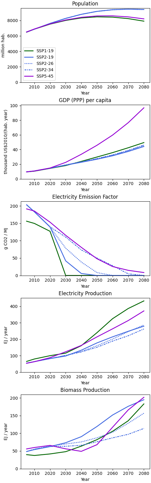
Not all data is required for air traffic estimation, only Population and GDP per capita. Now we interpolate, for each scenario, to get values yearly.
years = linspace(2024, 2080, 101)
population = {
    scenario: interpolate_data(
        years, np_array(years_data), np_array(scenario_data["population"][scenario])
    )
    for scenario in scenario_data["population"]
}
gdp_per_capita = {
    scenario: interpolate_data(
        years, np_array(years_data), np_array(scenario_data["gdp_per_capita"][scenario])
    )
    for scenario in scenario_data["gdp_per_capita"]
}
Also, we consider COVID effects by delaying trend traffic of a fixed amount of years, here we must also include the assumption of end of COVID related traffic constraints.
year_covid_end = 2024
gdp_per_capita_end_covid = {
    scenario: interpolate_data(
        year_covid_end,
        np_array(years_data),
        np_array(scenario_data["gdp_per_capita"][scenario]),
    )
    for scenario in scenario_data["gdp_per_capita"]
}
gdp_per_capita_2019 = {
    scenario: interpolate_data(
        2019.0,
        np_array(years_data),
        np_array(scenario_data["gdp_per_capita"][scenario]),
    )
    for scenario in scenario_data["gdp_per_capita"]
}
Model vectorization#
When a model must be evaluated yearly, rather than once, we must vectorize its function to account for vectorized inputs. When running a TemporalScenario this is done automatically, but here we must to it manually.
model = AirTraffic()
model.discipline.jax_out_func = vmap(model.discipline.jax_out_func)
Results#
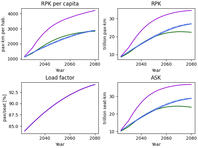
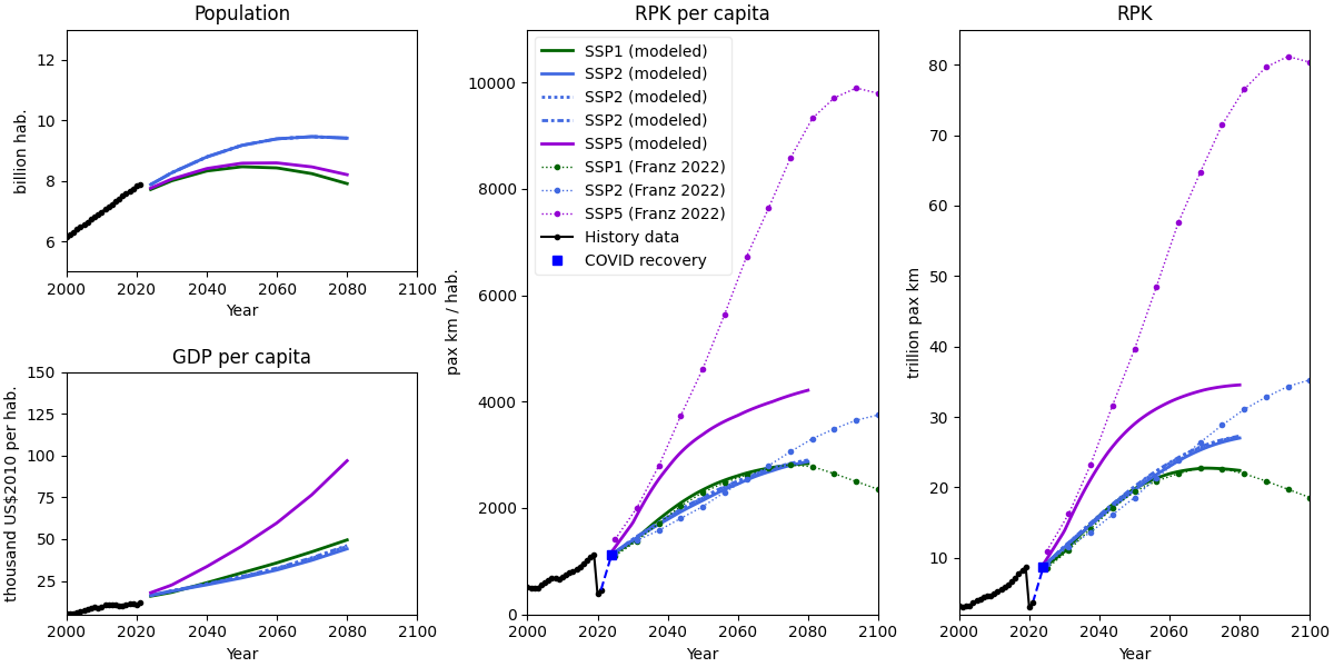
Now let’s visualize the results for each scenario Also we will make the paper plot with historical and COVID effects
outputs = {}
fig, axes = subplots(2, 2, layout="constrained")
vones = ones(years.shape)

years_hist, gdp_pc_hist, rpk_pc_hist, pop_hist = get_rpk_data(1970)
rpk_hist = rpk_pc_hist * pop_hist

fig_paper = figure(layout="constrained")

gs = fig_paper.add_gridspec(2, 3)
ax1 = fig_paper.add_subplot(gs[0, 0])
ax2 = fig_paper.add_subplot(gs[1, 0])
ax3 = fig_paper.add_subplot(gs[:, 1])
ax4 = fig_paper.add_subplot(gs[:, 2])

lines = lines_gen()
last_ssp_index = 0
for scenario in population:
    name_split = scenario.split("SSP")
    ssp_idx = int(name_split[1][0])
    if ssp_idx != last_ssp_index:
        lines = lines_gen()
    line = next(lines)
    last_ssp_index = ssp_idx

    capacity_factor = 1.0
    if ssp_idx == 1:
        capacity_factor = 0.9
    elif ssp_idx == 5:
        capacity_factor = 1.5

    model_input = {
        "year": years,
        "gdp_per_capita": gdp_per_capita[scenario],
        "population": population[scenario],
        "gdp_per_capita_covid_end": gdp_per_capita_end_covid[scenario] * vones,
        "gdp_per_capita_2019": gdp_per_capita_2019[scenario] * vones,
        "load_factor_end_year": 95.0 * vones,
        "end_year": 2100.0 * vones,
        "capacity_factor": capacity_factor * vones,
    }
    model_output = model.discipline.execute(model_input)
    outputs[scenario] = model_output

    axes[0, 0].plot(
        years,
        model_output["rpk_per_capita"],
        label=f"SSP{ssp_idx}",
        linestyle=line,
        color=get_scenario_color(scenario),
    )
    axes[0, 1].plot(
        years,
        1.0e-12 * model_output["rpk_trend"],
        linestyle=line,
        color=get_scenario_color(scenario),
    )
    axes[1, 0].plot(
        years,
        model_output["load_factor"],
        linestyle=line,
        color=get_scenario_color(scenario),
    )
    axes[1, 1].plot(
        years,
        1.0e-12 * model_output["ask_trend"],
        linestyle=line,
        color=get_scenario_color(scenario),
    )

    ax1.plot(
        years,
        population[scenario] * 1e-9,
        label=f"SSP{ssp_idx}",
        color=get_scenario_color(scenario),
        linestyle=line,
        linewidth=2,
    )
    ax2.plot(
        years,
        gdp_per_capita[scenario] * 1.0e-3,
        label=f"SSP{ssp_idx}",
        color=get_scenario_color(scenario),
        linestyle=line,
        linewidth=2,
    )
    ax3.plot(
        years,
        model_output["rpk_per_capita"],
        label=f"SSP{ssp_idx} (modeled)",
        color=get_scenario_color(scenario),
        linestyle=line,
        linewidth=2,
    )
    ax4.plot(
        years,
        model_output["rpk_trend"] * 1e-12,
        # label=f"SSP{ssp_idx}",
        color=get_scenario_color(scenario),
        linestyle=line,
        linewidth=2,
    )

axes[0, 0].set_xlabel("Year")
axes[0, 0].set_ylabel("pax-km per hab.")
axes[0, 0].set_title("RPK per capita")
axes[0, 1].set_xlabel("Year")
axes[0, 1].set_ylabel("trillion pax-km")
axes[0, 1].set_title("RPK")
axes[1, 0].set_xlabel("Year")
axes[1, 0].set_ylabel("pax/seat [%]")
axes[1, 0].set_title("Load factor")
axes[1, 1].set_xlabel("Year")
axes[1, 1].set_ylabel("trillion seat-km")
axes[1, 1].set_title("ASK")

fig_paper.set_size_inches(12, 6)
ax1.set_title("Population")
ax1.set_ylabel("billion hab.")
ax1.set_xlabel("Year")
ax1.set_xlim((2000, 2100))
ax1.set_ylim((5, 13))
ax2.set_title("GDP per capita")
ax2.set_ylabel("thousand US$2010 per hab.")
ax2.set_xlabel("Year")
ax2.set_xlim((2000, 2100))
ax2.set_ylim((5, 150))

ax3.plot(
    edge_time,
    1.0e12 * edge_ssp1 / interpolate_data(edge_time, years, population["SSP1-19"]),
    ":.",
    label="SSP1 (Franz 2022)",
    color=get_scenario_color("SSP1"),
    linewidth=1,
)
ax3.plot(
    edge_time,
    1.0e12 * edge_ssp2 / interpolate_data(edge_time, years, population["SSP2-26"]),
    ":.",
    label="SSP2 (Franz 2022)",
    color=get_scenario_color("SSP2"),
    linewidth=1,
)
ax3.plot(
    edge_time,
    1.0e12 * edge_ssp5 / interpolate_data(edge_time, years, population["SSP5-45"]),
    ":.",
    label="SSP5 (Franz 2022)",
    color=get_scenario_color("SSP5"),
    linewidth=1,
)
ax4.plot(
    edge_time,
    edge_ssp1,
    ":.",
    label="SSP1 (Franz 2022)",
    color=get_scenario_color("SSP1"),
    linewidth=1,
)
ax4.plot(
    edge_time,
    edge_ssp2,
    ":.",
    label="SSP2 (Franz 2022)",
    color=get_scenario_color("SSP2"),
    linewidth=1,
)
ax4.plot(
    edge_time,
    edge_ssp5,
    ":.",
    label="SSP5 (Franz 2022)",
    color=get_scenario_color("SSP5"),
    linewidth=1,
)

# ax4.legend(loc="upper left", framealpha=0.7)
ax4.set_title("RPK")
ax4.set_ylabel("trillion pax km")
ax4.set_xlabel("Year")
ax4.set_xlim((2000, 2100))
ax4.set_ylim((2, 85))

# Add hypothesis on COVID recovery
ax4.plot(
    [years_hist[-1], 2024],
    [rpk_hist[-1] * 1e6 * 1e-12, rpk_hist[-3] * 1e6 * 1e-12],
    "b--",
)
ax4.plot(
    2024,
    rpk_hist[-3] * 1e6 * 1e-12,
    "bs",
    # label="COVID recovery",
)

# Plot history
ax1.plot(
    years_hist,
    pop_hist * 1e-9,
    ".k",
    linestyle="-",
    label="History data",
)
ax2.plot(
    years_hist,
    gdp_pc_hist * 1.0e-3,
    ".k",
    linestyle="-",
    label="History data",
)
ax3.plot(
    years_hist,
    rpk_hist * 1.0e6 / pop_hist,
    "k.",
    linestyle="-",
    label="History data",
)

ax3.set_title("RPK per capita")
ax3.set_ylabel("pax km / hab.")
ax3.set_xlabel("Year")
ax3.set_xlim((2000, 2100))
ax3.set_ylim((0, 11000))

# Add hypothesis on COVID recovery
ax3.plot(
    [years_hist[-1], 2024],
    [rpk_hist[-1] * 1e6 / pop_hist[-1], rpk_hist[-3] * 1e6 / pop_hist[-3]],
    "b--",
)
ax3.plot(
    2024,
    rpk_hist[-3] * 1e6 / pop_hist[-3],
    "bs",
    label="COVID recovery",
)
ax3.legend(loc="upper left", framealpha=0.4)

ax4.plot(
    years_hist,
    rpk_hist * 1e6 * 1e-12,
    "k.",
    linestyle="-",
    # label="History data",
)

fig_paper.savefig("./rpk_ssps.pdf")
show()


# savefig(f"./rpk_summary.pdf")
# close(fig_paper)
Total running time of the script: (0 minutes 2.784 seconds)