Energy production system

from jax import vmap
from matplotlib.pyplot import show
from matplotlib.pyplot import subplots
from numpy import full
from numpy import interp
from numpy import linspace

from noads.application.background_scenario_data import get_ar6_input_data
from noads.application.base_objects import initialize_base_objects

Building the energy mix

The energy mix assembles the production graph of the paper: primary resources (oil, biomass, electricity), production pathways, and the energy carriers embarked in aircraft. Here we build it and evaluate its intensive models (impact and consumption per unit produced) over time, under the SSP2-2.6 background scenario.

BACKGROUND = "SSP2-26"

energy_mix, _fleet = initialize_base_objects(drop_in_only=False, technology_index=1)

years = linspace(2025.0, 2065.0, 41)


def find_energy(name):
    """Return a produced energy of the mix by name."""
    return next(e for e in energy_mix.produced_energies if e.name == name)

Scenario-dependent inputs

The emission factor of grid electricity comes from the AR6 scenario database, and the efficiencies of the electricity-based processes mature in time (2025, 2035, 2050 values, constant afterwards). The remaining coefficients are the constants of the energy pathway table of the paper.

ar6_data, years_data = get_ar6_input_data(
    start_year=2010, end_year=2080, plot_data=False
)
grid_ci = interp(years, years_data, ar6_data["ELECTRICITY.CO2_index"][BACKGROUND])


def maturing(v2025, v2035, v2050):
    """Interpolate a maturing coefficient onto the years vector."""
    return interp(years, [2025.0, 2035.0, 2050.0], [v2025, v2035, v2050])


data = {
    # Primary resource emission indices [g CO2 / MJ]
    "OIL.CO2_index": full(years.shape, 73.2 * 0.865),
    "BIOMASS.CO2_index": full(years.shape, 0.0),
    "ELECTRICITY.CO2_index": grid_ci,
    # Fossil kerosene
    "Refinery.direct.CO2_index": full(years.shape, 88.7 - 73.2),
    "Refinery.OIL.efficiency": full(years.shape, 0.865),
    # Biofuels [MJ biofuel / MJ biomass]
    "HEFA.direct.CO2_index": full(years.shape, 62.75),
    "HEFA.BIOMASS.efficiency": full(years.shape, 0.59),
    "FT.direct.CO2_index": full(years.shape, 35.3),
    "FT.BIOMASS.efficiency": full(years.shape, 0.20),
    "ATJ.direct.CO2_index": full(years.shape, 51.55),
    "ATJ.BIOMASS.efficiency": full(years.shape, 0.30),
    # Gaseous hydrogen (all from electrolysis here)
    "Electrolysis.direct.CO2_index": full(years.shape, 0.0),
    "Electrolysis.ELECTRICITY.efficiency": maturing(0.71, 0.71 * 1.03, 0.71 * 1.06),
    "Gas_reforming.direct.CO2_index": full(years.shape, 100.0),
    "Electrolysis.share": full(years.shape, 1.0),
    # Electrofuel
    "Power_to_liquid.direct.CO2_index": full(years.shape, 0.0),
    "Power_to_liquid.ELECTRICITY.efficiency": maturing(1.53, 1.53 * 1.08, 1.53 * 1.16),
    "Power_to_liquid.GAS-H2.efficiency": maturing(0.53, 0.53 * 1.06, 0.53 * 1.12),
    # Liquid hydrogen
    "H2_liquefaction.direct.CO2_index": full(years.shape, 0.0),
    "H2_liquefaction.GAS-H2.efficiency": full(years.shape, 1.0),
    "H2_liquefaction.ELECTRICITY.efficiency": maturing(4.54, 4.54 * 1.2, 4.54 * 1.4),
    # Batteries
    "Charging.direct.CO2_index": full(years.shape, 0.0),
    "Charging.ELECTRICITY.efficiency": full(years.shape, 0.98),
}

Evaluating the intensive chain

Impact indices are computed from primary to final energies: each pathway model adds the indirect impacts of its inputs to its direct impacts, and each energy model mixes its pathways. The models are plain JAX disciplines, so one vmap evaluates all the years at once.

gh2 = find_energy("GAS-H2")
chain = [
    find_energy("KEROSENE").pathways[0].impact_index_model(),  # Refinery
    *[pathway.impact_index_model() for pathway in find_energy("BIOFUEL").pathways],
    *[pathway.impact_index_model() for pathway in gh2.pathways],
    gh2.impact_index_model(),  # mixes electrolysis and gas reforming
    find_energy("E-FUEL").pathways[0].impact_index_model(),  # Power-to-liquid
    find_energy("LIQUID-H2").pathways[0].impact_index_model(),  # Liquefaction
    find_energy("BATTERY").pathways[0].impact_index_model(),  # Charging
]

for model in chain:
    model.discipline.jax_out_func = vmap(model.discipline.jax_out_func)
    inputs = {name: data[name] for name in model.discipline.input_grammar.names}
    data.update(model.discipline.execute(inputs))

Carbon intensity of the produced energies

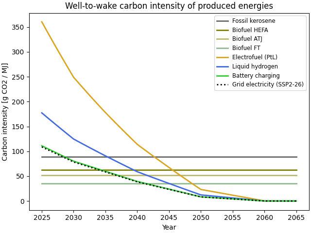
Fossil kerosene and biofuels have constant well-to-wake carbon intensities, while the electricity-based products (electrofuel, liquid hydrogen, battery charging) decarbonize with the background grid and with maturing process efficiencies.

carbon_intensities = {
    "Fossil kerosene": ("Refinery.CO2_index", "dimgray"),
    "Biofuel HEFA": ("HEFA.CO2_index", "olive"),
    "Biofuel ATJ": ("ATJ.CO2_index", "darkkhaki"),
    "Biofuel FT": ("FT.CO2_index", "darkseagreen"),
    "Electrofuel (PtL)": ("Power_to_liquid.CO2_index", "goldenrod"),
    "Liquid hydrogen": ("H2_liquefaction.CO2_index", "royalblue"),
    "Battery charging": ("Charging.CO2_index", "limegreen"),
}

fig1, ax1 = subplots(layout="constrained")
for label, (name, color) in carbon_intensities.items():
    ax1.plot(years, data[name], label=label, color=color, linewidth=2)
ax1.plot(years, grid_ci, "k:", label=f"Grid electricity ({BACKGROUND})", linewidth=2)
ax1.set_xlabel("Year")
ax1.set_ylabel("Carbon intensity [g CO2 / MJ]")
ax1.set_title("Well-to-wake carbon intensity of produced energies")
ax1.legend(fontsize="small")
show()

Biomass intensity of biofuels

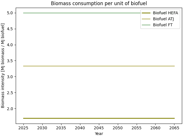
The biofuel pathways trade emissions against biomass use: HEFA emits the most but consumes the least biomass, Fischer-Tropsch the reverse.

biomass_intensity = {
    "Biofuel HEFA": ("HEFA.BIOMASS.consumption_index", "olive"),
    "Biofuel ATJ": ("ATJ.BIOMASS.consumption_index", "darkkhaki"),
    "Biofuel FT": ("FT.BIOMASS.consumption_index", "darkseagreen"),
}

fig2, ax2 = subplots(layout="constrained")
for label, (name, color) in biomass_intensity.items():
    ax2.plot(years, data[name], label=label, color=color, linewidth=2)
ax2.set_xlabel("Year")
ax2.set_ylabel("Biomass intensity [MJ biomass / MJ biofuel]")
ax2.set_title("Biomass consumption per unit of biofuel")
ax2.legend()
show()

Electricity intensity of the embarked energies

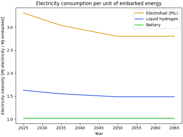
For the electricity-based carriers, the total (direct plus upstream) electricity consumed per MJ embarked is chained through gaseous hydrogen: electrofuel and liquid hydrogen consume electricity both directly and through electrolysis.

elec_per_gh2 = data["GAS-H2.ELECTRICITY.consumption_index"]
electricity_intensity = {
    "Electrofuel (PtL)": (
        data["Power_to_liquid.ELECTRICITY.consumption_index"]
        + data["Power_to_liquid.GAS-H2.consumption_index"] * elec_per_gh2,
        "goldenrod",
    ),
    "Liquid hydrogen": (
        data["H2_liquefaction.ELECTRICITY.consumption_index"]
        + data["H2_liquefaction.GAS-H2.consumption_index"] * elec_per_gh2,
        "royalblue",
    ),
    "Battery": (data["Charging.ELECTRICITY.consumption_index"], "limegreen"),
}

fig3, ax3 = subplots(layout="constrained")
for label, (values, color) in electricity_intensity.items():
    ax3.plot(years, values, label=label, color=color, linewidth=2)
ax3.set_xlabel("Year")
ax3.set_ylabel("Electricity intensity [MJ electricity / MJ embarked]")
ax3.set_title("Electricity consumption per unit of embarked energy")
ax3.legend()
show()

Carbon intensity versus resource intensity

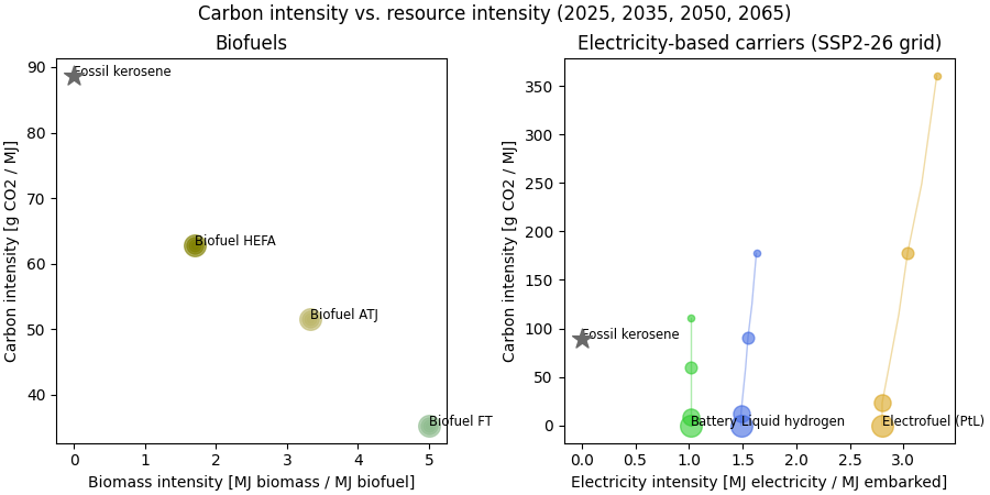
The trade-off between climate impact and resource consumption, evaluated at 2025, 2035, 2050, and 2065. The biofuel pathways are fixed points; the electricity-based carriers move down-left as the grid decarbonizes and the processes mature (marker size grows with the year).

snapshot_years = [2025.0, 2035.0, 2050.0, 2065.0]
snapshots = [int((y - years[0]) / (years[1] - years[0])) for y in snapshot_years]
sizes = [20, 60, 120, 200]

fig4, (ax_bio, ax_elec) = subplots(1, 2, figsize=(9, 4.5), layout="constrained")

# Fossil kerosene is the reference: it consumes neither biomass nor electricity,
# so it sits on the vertical axis of both panels at its constant carbon intensity.
kerosene_ci = float(data["Refinery.CO2_index"][0])

for label, (name, color) in biomass_intensity.items():
    ci = data[label.replace("Biofuel ", "") + ".CO2_index"]
    for i, size in zip(snapshots, sizes):
        ax_bio.scatter(data[name][i], ci[i], s=size, color=color, alpha=0.6)
    ax_bio.annotate(label, (data[name][-1], ci[-1]), fontsize="small")
ax_bio.scatter(0.0, kerosene_ci, marker="*", s=180, color="dimgray", zorder=5)
ax_bio.annotate("Fossil kerosene", (0.0, kerosene_ci), fontsize="small")
ax_bio.set_xlabel("Biomass intensity [MJ biomass / MJ biofuel]")
ax_bio.set_ylabel("Carbon intensity [g CO2 / MJ]")
ax_bio.set_title("Biofuels")

ci_names = {
    "Electrofuel (PtL)": "Power_to_liquid.CO2_index",
    "Liquid hydrogen": "H2_liquefaction.CO2_index",
    "Battery": "Charging.CO2_index",
}
for label, (values, color) in electricity_intensity.items():
    ci = data[ci_names[label]]
    ax_elec.plot(values, ci, color=color, alpha=0.4, linewidth=1)
    for i, size in zip(snapshots, sizes):
        ax_elec.scatter(values[i], ci[i], s=size, color=color, alpha=0.6)
    ax_elec.annotate(label, (values[-1], ci[-1]), fontsize="small")
ax_elec.scatter(0.0, kerosene_ci, marker="*", s=180, color="dimgray", zorder=5)
ax_elec.annotate("Fossil kerosene", (0.0, kerosene_ci), fontsize="small")
ax_elec.set_xlabel("Electricity intensity [MJ electricity / MJ embarked]")
ax_elec.set_ylabel("Carbon intensity [g CO2 / MJ]")
ax_elec.set_title(f"Electricity-based carriers ({BACKGROUND} grid)")

fig4.suptitle("Carbon intensity vs. resource intensity (2025, 2035, 2050, 2065)")
show()