Time-dependent controls and the first-order delay

from matplotlib.pyplot import show
from matplotlib.pyplot import subplots
from numpy import array
from numpy import interp
from numpy import linspace
from scipy.integrate import solve_ivp

The first-order delay

Every time-dependent optimization variable (a control) enters the simulation through a first-order delay, which turns a possibly abrupt decision into a gradual response and improves the stability and dimensionality of the optimization. The delayed output o(t) follows the input signal i(t) with a time constant tau:

\[\frac{d}{dt}o(t) = \frac{i(t) - o(t)}{\tau}\]

The helper below integrates that equation (mirroring noads.core.scenarios.temporalscenario.delay1_rhs), with the input signal given as (times, values) knots interpolated linearly, and an initial output of zero.

def first_order_delay(times, values, tau, t_eval):
    """Response of the first-order delay to a piecewise-linear input signal."""
    times, values = array(times, dtype=float), array(values, dtype=float)

    def rhs(t, o):
        return (interp(t, times, values) - o) / tau

    solution = solve_ivp(
        rhs, (t_eval[0], t_eval[-1]), [0.0], t_eval=t_eval, max_step=0.25
    )
    return solution.y[0]

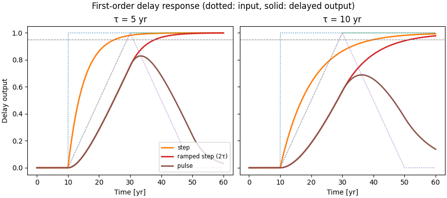
Response to a step, a ramped step, and a pulse, for two time constants. For a ramped step of ramp duration 2*tau the output reaches 95 % of its target after about 4*tau, which the model interprets as one fleet-replacement lifetime.

t = linspace(0, 60, 601)
inputs = {
    "step": ([0, 10, 10.001, 60], [0, 0, 1, 1]),
    "ramped step (2τ)": ([0, 10, 30, 60], [0, 0, 1, 1]),
    "pulse": ([0, 10, 30, 50, 60], [0, 0, 1, 0, 0]),
}

fig1, axes1 = subplots(1, 2, figsize=(9, 4), layout="constrained", sharey=True)
for ax, tau in zip(axes1, (5.0, 10.0)):
    for label, (times, values) in inputs.items():
        ax.plot(t, interp(t, times, values), ":", linewidth=1)
        ax.plot(t, first_order_delay(times, values, tau, t), label=label, linewidth=2)
    ax.axhline(0.95, color="gray", linewidth=0.8, linestyle="--")
    ax.set_title(f"τ = {tau:.0f} yr")
    ax.set_xlabel("Time [yr]")
axes1[0].set_ylabel("Delay output")
axes1[0].legend(loc="lower right", fontsize="small")
fig1.suptitle("First-order delay response (dotted: input, solid: delayed output)")
show()

years = linspace(2025, 2075, 501)


def ramped_pulse(eis, max_share, ramp_up=5.0, lifetime=25.0, ramp_down=5.0):
    """Trapezoidal market-share input, as built in ``AircraftDesign._control_share``."""
    times = [eis, eis + ramp_up, eis + lifetime, eis + lifetime + ramp_down]
    return times, [0.0, max_share, max_share, 0.0]

Aircraft market share — a valid market mix

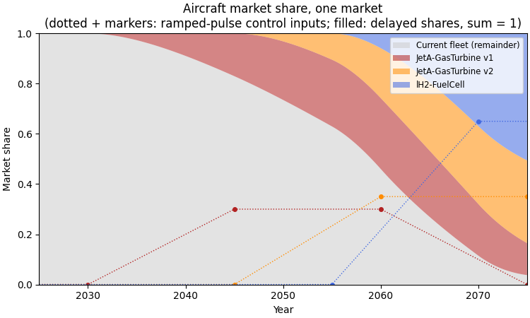
Within a market, each new aircraft’s share is a ramped pulse set by four optimization variables (Entry-Into-Service, maximum share, lifetime, ramp-down) with delay tau = market_lifetime / 4. The control constraint is that the new-aircraft shares sum to at most one at every time, the current fleet taking the remainder (1 - sum). The configuration below respects it: the delayed shares stack up to one, so the current-fleet remainder stays non-negative. Dotted lines with markers are the ramped-pulse control inputs; the filled areas are the delayed shares.

market_lifetime = 30.0
tau_fleet = market_lifetime / 4.0
new_aircraft = {
    "JetA-GasTurbine v1": {"eis": 2030, "max_share": 0.3, "color": "firebrick"},
    "JetA-GasTurbine v2": {"eis": 2045, "max_share": 0.35, "color": "darkorange"},
    "lH2-FuelCell": {"eis": 2055, "max_share": 0.65, "color": "royalblue"},
}

fig2, ax2 = subplots(figsize=(7.5, 4.5), layout="constrained")
delayed_shares = []
for cfg in new_aircraft.values():
    times, values = ramped_pulse(
        cfg["eis"],
        cfg["max_share"],
        ramp_up=2 * tau_fleet,
        lifetime=market_lifetime,
        ramp_down=2 * tau_fleet,
    )
    delayed_shares.append(first_order_delay(times, values, tau_fleet, years))
    ax2.plot(years, interp(years, times, values), ":", color=cfg["color"], linewidth=1)
    ax2.plot(times, values, "o", color=cfg["color"], markersize=4)

stack = array(delayed_shares)
current_fleet = 1.0 - stack.sum(axis=0)
assert (stack.sum(axis=0) <= 1.0 + 1e-9).all(), "aircraft shares exceed 1"
ax2.stackplot(
    years,
    current_fleet,
    *stack,
    labels=["Current fleet (remainder)", *new_aircraft],
    colors=["0.8", *[cfg["color"] for cfg in new_aircraft.values()]],
    alpha=0.55,
)
ax2.set_xlabel("Year")
ax2.set_ylabel("Market share")
ax2.set_ylim(0, 1)
ax2.set_xlim(2025, 2075)
ax2.set_title(
    "Aircraft market share, one market\n"
    "(dotted + markers: ramped-pulse control inputs; filled: delayed shares, sum = 1)"
)
ax2.legend(loc="upper right", fontsize="small")
show()

Energy pathway shares — a valid mix

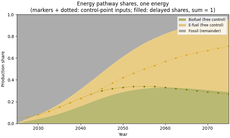
The shares of the pathways producing one energy are knot controls (their values at every 2.5 years are optimization variables), with delay tau = 5 yr. The constraint is that the shares are non-negative and sum to one, so the last pathway takes the remainder. The two free controls below stay non-negative and sum to at most one at every knot, keeping the remainder valid.

knots = linspace(2025, 2075, 21)
share_bio = array([
    0.05,
    0.06,
    0.08,
    0.11,
    0.15,
    0.19,
    0.23,
    0.27,
    0.30,
    0.32,
    0.33,
    0.34,
    0.34,
    0.34,
    0.33,
    0.32,
    0.31,
    0.30,
    0.29,
    0.28,
    0.27,
])  # noqa: E501
share_efuel = array([
    0.05,
    0.06,
    0.08,
    0.11,
    0.15,
    0.19,
    0.23,
    0.27,
    0.32,
    0.37,
    0.42,
    0.46,
    0.50,
    0.53,
    0.57,
    0.60,
    0.63,
    0.65,
    0.67,
    0.69,
    0.71,
])  # noqa: E501
assert ((share_bio + share_efuel) <= 1.0).all(), "pathway shares exceed 1"

delayed_bio = first_order_delay(knots, share_bio, 5.0, years)
delayed_efuel = first_order_delay(knots, share_efuel, 5.0, years)
delayed_fossil = 1.0 - delayed_bio - delayed_efuel

fig3, ax3 = subplots(figsize=(7.5, 4.5), layout="constrained")
for knot_values, color in [(share_bio, "olive"), (share_efuel, "goldenrod")]:
    ax3.plot(knots, knot_values, "o", color=color, markersize=3)
    ax3.plot(years, interp(years, knots, knot_values), ":", color=color, linewidth=1)
ax3.stackplot(
    years,
    delayed_bio,
    delayed_efuel,
    delayed_fossil,
    labels=["Biofuel (free control)", "E-fuel (free control)", "Fossil (remainder)"],
    colors=["olive", "goldenrod", "dimgray"],
    alpha=0.55,
)
ax3.set_xlabel("Year")
ax3.set_ylabel("Production share")
ax3.set_ylim(0, 1)
ax3.set_xlim(2025, 2075)
ax3.set_title(
    "Energy pathway shares, one energy\n"
    "(markers + dotted: control-point inputs; filled: delayed shares, sum = 1)"
)
ax3.legend(loc="upper right", fontsize="small")
show()

Demand avoidance — a valid supply-shift ratio

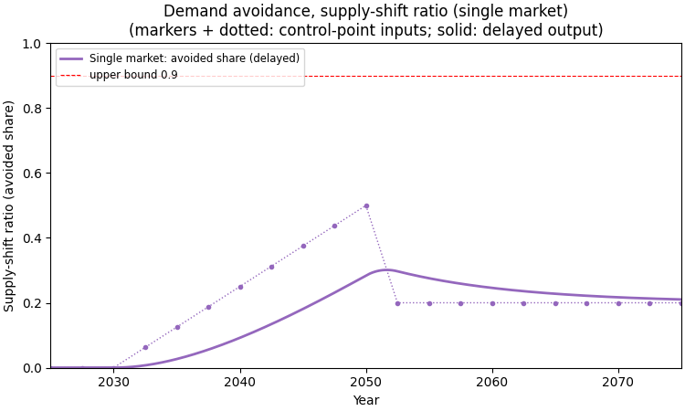
In the low-demand formulation each market has a supply-shift ratio control – the fraction of trend supply that is avoided – with knot values (every 2.5 years, as optimization variables) bounded to [0, 0.9] and delay tau = 10 yr. The delayed control is the realised avoidance; 1 - SR is the fraction of trend traffic still served. A single market is shown: the supply-shift ratio ramps linearly from 0 to 0.5 between 2030 and 2050, then drops to 0.2 and stays there.

sr_knots = linspace(2025, 2075, 21)
sr_market = array([
    0.0,
    0.0,
    0.0,
    0.0625,
    0.125,
    0.1875,
    0.25,
    0.3125,
    0.375,
    0.4375,
    0.5,
    0.2,
    0.2,
    0.2,
    0.2,
    0.2,
    0.2,
    0.2,
    0.2,
    0.2,
    0.2,
])  # noqa: E501
assert (sr_market >= 0.0).all(), "supply-shift ratio below 0"
assert (sr_market <= 0.9).all(), "supply-shift ratio above 0.9"

fig4, ax4 = subplots(figsize=(7.5, 4.5), layout="constrained")
ax4.plot(sr_knots, sr_market, "o", color="C4", markersize=3)
ax4.plot(years, interp(years, sr_knots, sr_market), ":", color="C4", linewidth=1)
ax4.plot(
    years,
    first_order_delay(sr_knots, sr_market, 10.0, years),
    color="C4",
    linewidth=2,
    label="Single market: avoided share (delayed)",
)
ax4.axhline(0.9, color="red", linewidth=0.8, linestyle="--", label="upper bound 0.9")
ax4.set_xlabel("Year")
ax4.set_ylabel("Supply-shift ratio (avoided share)")
ax4.set_ylim(0, 1)
ax4.set_xlim(2025, 2075)
ax4.set_title(
    "Demand avoidance, supply-shift ratio (single market)\n"
    "(markers + dotted: control-point inputs; solid: delayed output)"
)
ax4.legend(loc="upper left", fontsize="small")
show()